Disclaimer: The post is more about understanding LUTs and HaldCLUTs and writing methods from scratch to apply these LUTs to an image rather than coming up with CLUTs themselves from scratch.
Outline
- What are film simulations?
- CLUTs primer
- Simple hand-crafted CLUTs
- The identity CLUT
- HaldCLUTs
- Applying a HaldCLUT
- Notes and further reading
There is also an accompanying notebook, in case you want to play around with the CLUTs.
What are film simulations?
Apparently, back in the day, people shot pictures with analog cameras that used film. If you wanted a different “look” to your pictures, you would load a different film stock that gave you the desired look. This is akin to current-day Instagram filters, though more laborious. Some digital camera makers, like Fujifilm, started out as makers of photographic films (and they still make them), and transitioned into making digital cameras. Modern mirrorless cameras from Fujifilm have film simulation presets that digitally mimic the style of a particular film stock. If you are curious, John Peltier has written a good piece on Fujifilm’s film simulations. I was intrigued by how these simulations were achieved and this is a modest attempt at untangling them.
CLUTs primer
A CLUT, or a Color Look Up Table, is the primary way to define a style or film simulation. For each possible RGB color, a CLUT tells you which color to map it to. For example, a CLUT might specify that all green pixels in an image should be yellow:
# map green to yellow
(0, 255, 0) -> (255, 255, 0)
The actual format in which this information is represented can vary. A CLUT can be a .cube file, a HaldCLUT png, or even a pickled numpy array as long as whatever image editing software you use can read it.
In an 8-bit image, each channel (i.e red, green or blue) can take values from 0 to 255. Our CLUT should theoretically have a mapping for every possible color – that’s 256 x 256 x 256 colors. In practice however, CLUTs are way smaller. For example an 8-bit CLUT would divide each channel into ranges of 32 (i.e 256 divided by 8). Since we have 3 channels (red, green and blue), our CLUT can be imagined as a three dimensional cube:

To apply a CLUT to the image, each color in the image is assigned to one of the cells in the CLUT cube, and the color of the pixel in the original image is changed to whatever RGB color is in its assigned cell in the CLUT cube. Hence the color (12, 0, 0) would belong to the second cell along the red axis in the top left corner of the cube. This also means that all the shades of red between (8, 0, 0) and (15, 0, 0) will be mapped to the same RGB color. Though that sounds terrible, an 8-bit CLUT usually produces images that are fine to our eyes. Of course we can increase the “quality” of the resulting image by using a more precise (eg: 12-bit) CLUT.
Simple hand-crafted CLUTs
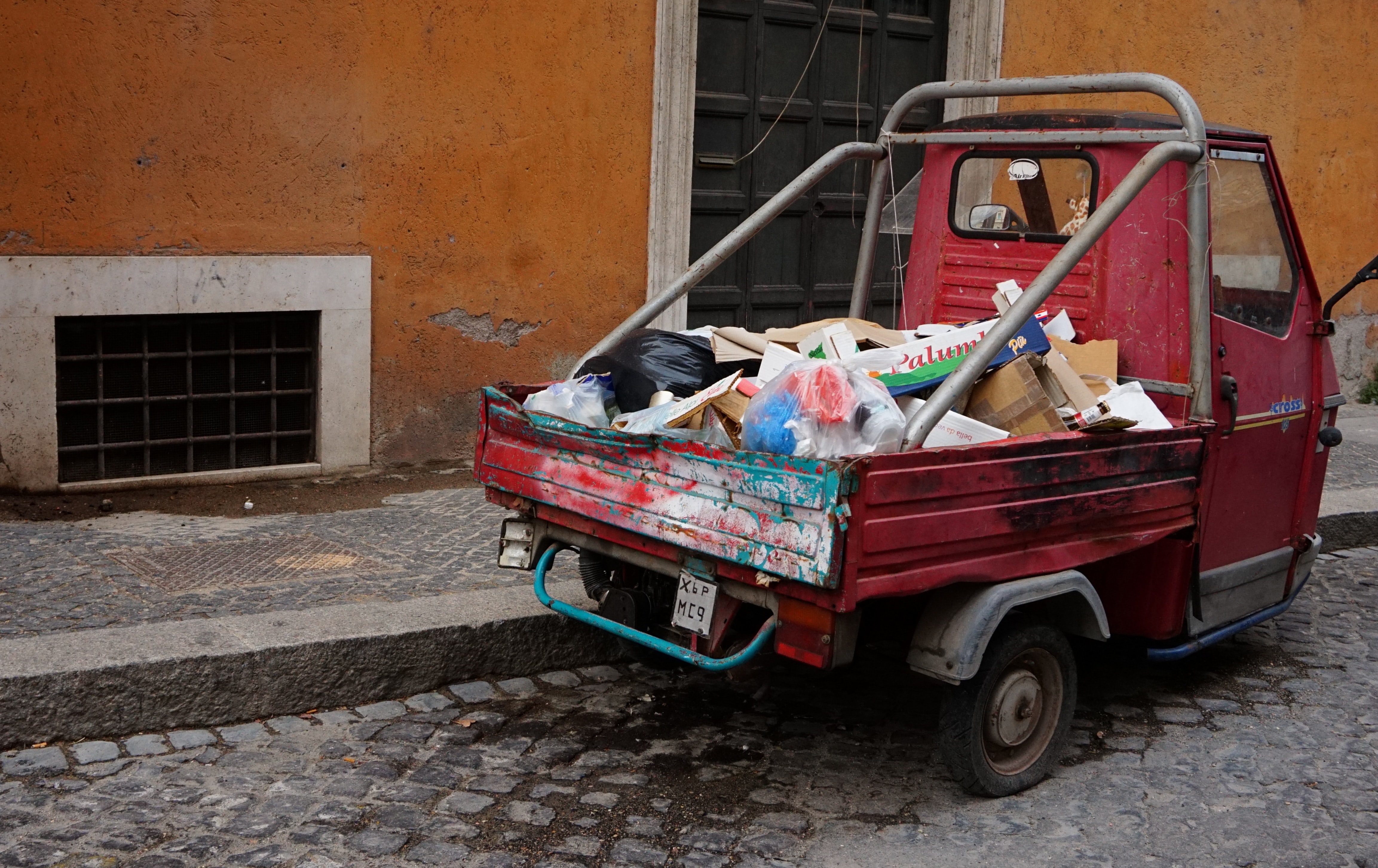
Before we craft CLUTs and start applying them to images, we need a test image. For the sake of simplicity, we conjure up a little red square:
from PIL import Image
img = Image.new('RGB', (60, 60), color='red')
img.show()

We will now create a simple CLUT that would map red pixels to green pixels and apply it to our little red square. We know that our CLUT should be a cube, and each “cell” in the cube should map to a color. If we create a 2-bit CLUT, it will have the shape (2, 2, 2, 3). Remember that our CLUT is a cube with each side of “length” 2, and that each “cell” in the cube should hold an RGB color – hence the 3 in the last dimension.
import numpy as np
clut = np.zeros((2, 2, 2, 3))
transformed_img = apply_3d_clut(clut, img, clut_size=2)
transformed_img.show()
We haven’t yet implemented the “apply_3d_clut()” method. This method will have to look at every pixel in the image and figure out the corresponding mapped pixel from the CLUT. The logic is roughly as follows:
- For each pixel in the image:
- get the (r, g, b) values for the pixel
- Assign the (r, g, b) values to a “cell” in our CLUT
- Replace the pixel in the original with the color in the assigned CLUT “cell”
We should be careful with step 2 above – since we have a 2-bit CLUT, we want color values up to 127 to be mapped to the first cell and we want values 127 and above to be mapped to the second cell.
from tqdm import tqdm
def apply_3d_clut(clut, img, clut_size=2):
    """
        clut must have the shape (size, size, size, num_channels)
    """
    num_rows, num_cols = img.size
    filtered_img = np.copy(np.asarray(img))
    scale = (clut_size - 1) / 255
    img = np.asarray(img)
    for row in tqdm(range(num_rows)):
        for col in range(num_cols):
            r, g, b = img[col, row]
            # (clut_r, clut_g, clut_b) together represents a "cell" in the CLUT
            # Notice that we rely on round() to map the values to "cells" in the CLUT
            clut_r, clut_g, clut_b = round(r * scale), round(g * scale), round(b * scale)
            # copy over the color in the CLUT to the new image
            filtered_img[col, row] = clut[clut_r, clut_g, clut_b]
    filtered_img = Image.fromarray(filtered_img.astype('uint8'), 'RGB')

    return filtered_img
Once you implement the above method and apply the CLUT to our image, you will be treated with a very underwhelming little black box:

Our CLUT was all zeros, and unsurprisingly, the red pixels in our little red square was mapped to black when the CLUT was applied. Let us now manipulate the CLUT to map red to green:
clut[1, 0, 0] = np.array([0, 255, 0])
transformed_img = apply_3d_clut(clut, img, clut_size=2)
transformed_img.show()

Fantastic, that worked! Time to apply our CLUT to a real image:

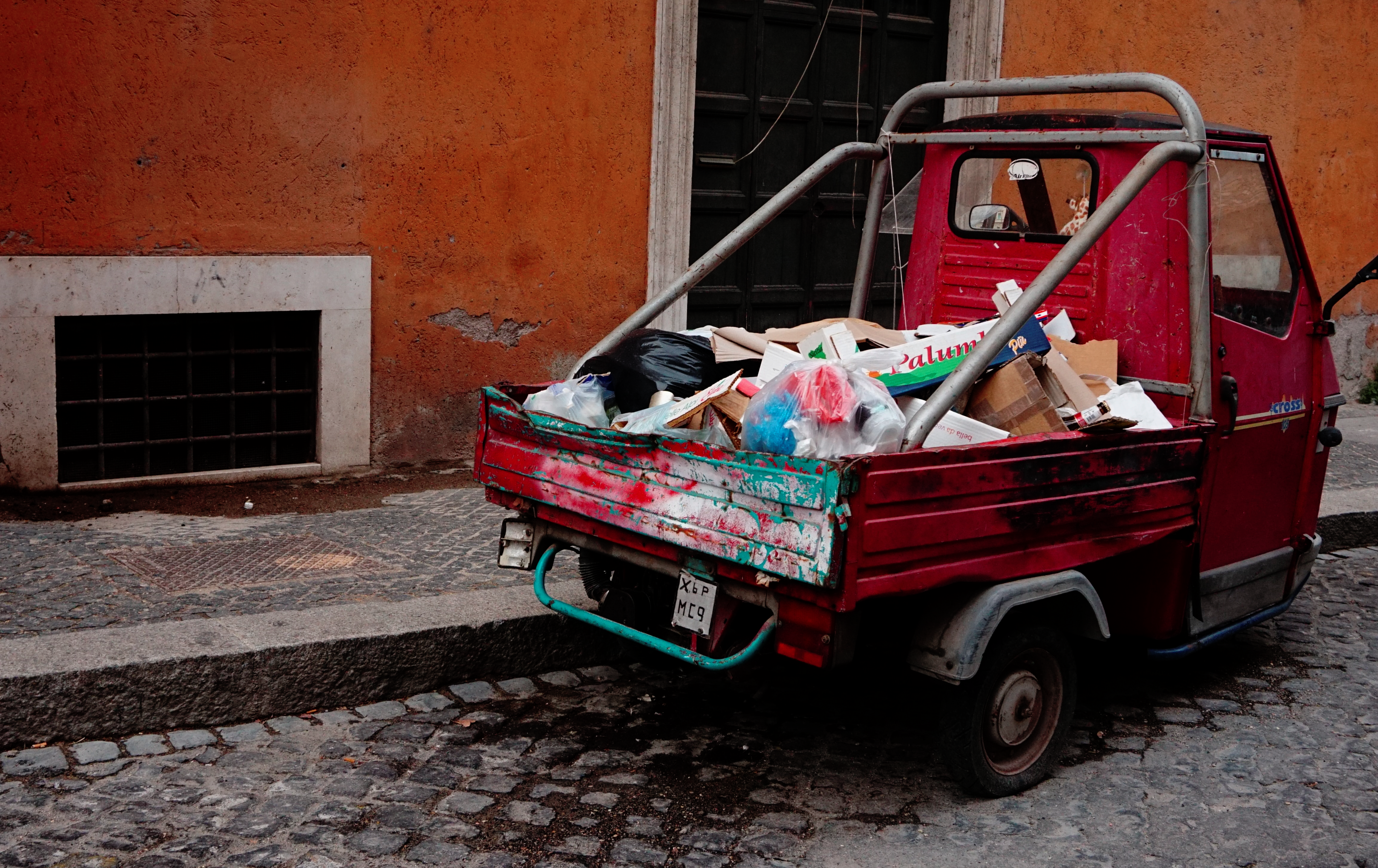
import urllib.request
truck = Image.open(urllib.request.urlopen("https://i.imgur.com/ahpSmLP.jpg"))
green_truck = apply_3d_clut(clut, truck, clut_size=2)
green_truck.show()

That’s a bit too green. We can see that the reds in the original image did get replaced by green pixels, but since we initialized our CLUT to all zeroes, all the other colors in the image was replaced with black pixels. We need a CLUT that would map all the reds to greens while leaving all the other colors alone.
Before we do that, let us vectorize our “apply_3d_lut()” method to make it much faster:
def fast_apply_3d_clut(clut, clut_size, img):
    """
        clut must have the shape (size, size, size, num_channels)
    """
    num_rows, num_cols = img.size
    filtered_img = np.copy(np.asarray(img))
    scale = (clut_size - 1) / 255
    img = np.asarray(img)
    clut_r = np.rint(img[:, :, 0] * scale).astype(int)
    clut_g = np.rint(img[:, :, 1] * scale).astype(int)
    clut_b = np.rint(img[:, :, 2] * scale).astype(int)
    filtered_img = clut[clut_r, clut_g, clut_b]
    filtered_img = Image.fromarray(filtered_img.astype('uint8'), 'RGB')
    return filtered_img
The identity CLUT
An identity CLUT, when applied, produces an image identical to the source image. In other words, the identity CLUT maps each color in the source image to the same color. The identity CLUT is a perfect base for us to build upon – we can change parts of the identity CLUT to manipulate certain colors while other colors in the image are left unchanged.
def create_identity(size):
    clut = np.zeros((size, size, size, 3))
    scale = 255 / (size - 1)
    for b in range(size):
        for g in range(size):
            for r in range(size):
                clut[r, g, b, 0] = r * scale
                clut[r, g, b, 1] = g * scale
                clut[r, g, b, 2] = b * scale
    return clut
Let us generate a 2-bit identity CLUT and see how applying it affects our image
two_bit_identity_clut = create_identity(2)
identity_truck = fast_apply_3d_clut(two_bit_identity_clut, 2, truck)
identity_truck = Image.fromarray(identity_truck.astype('uint8'), 'RGB')
identity_truck.show()

That’s in the same ballpark as the original image, but clearly there’s a lot wrong there. The problem is our 2-bit CLUT – we had a palette of only 8 colors (2 * 2 * 2) to choose from. Let us try again, but this time with a 12-bit CLUT:
twelve_bit_identity_clut = create_identity(12)
identity_truck = fast_apply_3d_clut(twelve_bit_identity_clut, 12, truck)
identity_truck = Image.fromarray(identity_truck.astype('uint8'), 'RGB')
identity_truck.show()
That’s much better. In fact, I can see no discernible differences between the images. Wunderbar!
Let us try mapping the reds to the greens again. Our goal is to map all pixels that are sufficiently red to green. What’s “sufficiently red”? For our purposes, all pixels that end up being mapped to the reddish corner of the CLUT cube deserve to be green.
green_clut = create_identity(12)
green_clut[5:, :4, :4] = np.array([0, 255, 0])
green_truck = fast_apply_3d_clut(green_clut, 12, truck)
green_truck.show()

That’s comically bad. Of course, we got what we asked for – some reddish parts of the image did get mapped to a bright ugly green. Let us restore our faith in CLUTs by attempting a slightly less drastic and potentially pleasing effect – make all pixels slightly more green:
green_clut = create_identity(12)
green_clut[:, :, :, 1] += 20
green_truck = fast_apply_3d_clut(green_clut, 12, truck)
green_truck.show()

Slightly less catastrophic. But we didn’t need CLUTs for this – we could have simply looped through all the pixels and manually added a constant value to the green channel. Theoretically, we can get more pleasing effects by fancier manipulation of the CLUT – instead of adding a constant value, maybe add a higher value to the reds and a lower value to the whites? You can probably see where this is going – coming up with good CLUTs (at least programmatically) is not trivial.
What do we do now? Let’s get us some professionally created CLUTs.
HaldCLUTs
We are going to apply the “Fuji Velvia 50” CLUT that is bundled with RawTherapee to our truck image. These CLUTs are distributed as HaldCLUT png files, and we will spend a few minutes understanding the format before writing a method to apply a HaldCLUT to the truck. But why HaldCLUTs?
- HaldCLUTs are high-fidelity. Our 12-bit identity CLUT was good enough to reproduce the image. Each HaldCLUT bundled with RawTherapee is equivalent to a 144-bit 3d CLUT. Yes, that’s effectively CLUT of shape (144, 144, 144, 3).
- However, the real benefit of using HaldCLUTs is the file size. Adobe’s .cube CLUT format is essentially a plain text file with RGB values. Since each character in the text file takes up a byte, a 144-bit CLUT in .cube takes up around 32MB on disk. The equivalent HaldCLUT png image file is around a megabyte. But png images are two-dimensional. How can we encode three-dimensional data using a two-dimensional image? We’ll see.
Let’s look at an identity HaldCLUT:

convert hald:12 -depth 8 -colorspace sRGB hald_12.png Pretty pretty colors. You’d have noticed that the image seems to have been divided into little cells. Let’s zoom in on the cell on the top-left corner:

We notice a few things – the pixel on the top-left is definitely black – so it represents the first “bucket” or “cell” in a 3D clut and pure blacks (i.e rgb(0, 0, 0)) are going to be mapped to the color present in this bucket . Of course the pixel at (0, 0, 0) in the above image is black because we are dealing with an identity CLUT here – a different CLUT could have mapped the index (0, 0, 0) to gray. The confusing part here is to figure out how to index into the HaldCLUT – let’s say we have a bright red pixel with the value (200, 0, 0) in our source image. If we were dealing with a normal 144-bit 3D CLUT, we would know that a red value of 200 will belong to the index 200 * 144 / 255 = 133 (approximately), and we would replace the color of this pixel with whatever was at CLUT[113][0][0]. But we are not dealing with a 3D CLUT here – we are dealing with a 2-D image, while we have to index into this image as if it was a 3D CLUT.
The entire identity HaldCLUT image in our example has the shape (1728, 1728), and each of those little cells that you see has the shape (12, 144), and there are 144 such cells in a single column of the image (i.e vertically). The HaldCLUT, as you can see, has 12 columns. Hence we have 1728 cells in the entire HaldCLUT, each cell having the shape (12, 144). This is how we index into a HaldCLUT file:
(if the description doesn’t make much sense, it is followed by a code snippet that’s hopefully clearer)
- Within each cell, the red index always changes from left to right. In our top-left cell, it changes from 0 to 143. This is the case in each row within each cell – the red index is always 0 in the first column of a cell, and 1 in the second column and so on. Since each cell has 12 rows, in each of these rows the red index changes from 0 to 143.
- The green index is constant in each row within a cell, and increments by 1 across cells horizontally, and wraps around. So the pixel at position (143, 0) in the HaldCLUT image represents the index
(143, 0, 0), while the pixel at position(144, 0)represents the index(0, 1, 0)and so on. The pixel at position(1, 0)would represent the index(0, 12, 0). - The blue channel is constant everywhere within a cell, and increments by 1 across cells vertically. So the pixel at position
(11, 0)will represent the index(0, 131, 0)while the pixel at(12, 0)will represent the index(0, 0, 1). Notice how both the red-index and green-index was reset to 0 when moved down the HaldCLUT image by an entire cell.
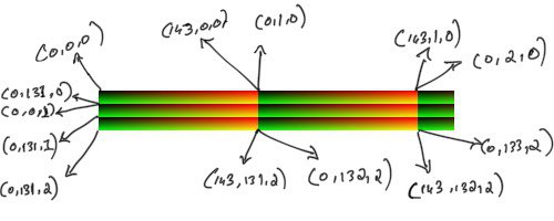
(12, 144). When there are two lines in the diagram seemingly coming out from the same pixel, I am trying to show how the represented index changes between adjacent pixels at a cell boundary. Inspecting the identity HaldCLUT in python reveals the same info:
identity = Image.open("identity.png")
identity = np.asarray(identity)
print("identity HaldCLUT has size: {}".format(identity.shape))
size = round(math.pow(identity.shape[0], 1/3))
print("The CLUT size is {}".format(size))
# The CLUT size is 12
print("clut[0,0] is {}".format(identity[0, 0]))
# clut[0,0] is [0 0 0]
print("clut[0, 100] is {}".format(identity[0, 100]))
# clut[0, 100] is [179   0   0]
print("clut[0, 143] is {}".format(identity[0, 143]))
# We've reached the end of the first row in the first cell
# clut[0, 143] is [255   0   0]
print("clut[0, 144] is {}".format(identity[0, 144]))
# The red channel resets, the green channel increments by 1
# clut[0, 144] is [0 1 0]
print("clut[0, 248] is {}".format(identity[0, 248]))
# clut[0, 248] is [186   1   0]
# Notice how the value in the green channel did not increase. This is normal - we have 256 possible values and only 144 "slots" to keep them. The identity CLUT occasionally skips a
print("clut[0, 432] is {}".format(identity[0, 432]))
# clut[0, 432] is [0 5 0]
# ^ The red got reset, the CLUT skipped more values in the green channel and now maps to 5. This is the peculiarity of this CLUT. A different HaldCLUT (not the identity one) might have had a different value for this green channel step.
print("clut[0, 1727] is {}".format(identity[0, 1727]))
# clut[0, 1727] is [255  19   0]
# This is the last pixel in the first row of the entire image
print("clut[1, 0] is {}".format(identity[1, 0]))
# clut[1, 0] is [ 0 21  0]
# Notice how the value in the green channel "wrapped around" from the previous row
print("clut[1, 144] is {}".format(identity[1, 144]))
# Exercise for the reader: see if you can guess the output correctly 🙂
print("clut[12 0] is {}".format(identity[12, 0]))
print("clut[12 143] is {}".format(identity[12, 143]))
print("clut[12 144] is {}".format(identity[12, 144]))
Applying a HaldCLUT
Now that we’ve understood how a 3D CLUT is sorta encoded in a HaldCLUT png, let’s go ahead and write a method to apply a HaldCLUT to an image:
import math
def apply_hald_clut(hald_img, img):
    hald_w, hald_h = hald_img.size
    clut_size = int(round(math.pow(hald_w, 1/3)))
    # We square the clut_size because a 12-bit HaldCLUT has the same amount of information as a 144-bit 3D CLUT
    scale = (clut_size * clut_size - 1) / 255
    # Convert the PIL image to numpy array
    img = np.asarray(img)
    # We are reshaping to (144 * 144 * 144, 3) - it helps with indexing
    hald_img = np.asarray(hald_img).reshape(clut_size ** 6, 3)
    # Figure out the 3D CLUT indexes corresponding to the pixels in our image
    clut_r = np.rint(img[:, :, 0] * scale).astype(int)
    clut_g = np.rint(img[:, :, 1] * scale).astype(int)
    clut_b = np.rint(img[:, :, 2] * scale).astype(int)
    filtered_image = np.zeros((img.shape))
    # Convert the 3D CLUT indexes into indexes for our HaldCLUT numpy array and copy over the colors to the new image
    filtered_image[:, :] = hald_img[clut_r + clut_size ** 2 * clut_g + clut_size ** 4 * clut_b]
    filtered_image = Image.fromarray(filtered_image.astype('uint8'), 'RGB')
    return filtered_image
Let’s test our method by applying the identity HaldCLUT to our truck – we should get a visually unchanged image back:
identity_hald_clut = Image.open(urllib.request.urlopen("https://i.imgur.com/qg6Is0w.png"))
identity_truck = apply_hald_clut(identity_hald_clut, truck)
identity_truck.show()
Let us finally apply the “Fuji Velvia 50” CLUT to our truck:
velvia_hald_clut = Image.open(urllib.request.urlopen("https://i.imgur.com/31UrdAg.png"))
velvia_truck = apply_hald_clut(velvia_hald_clut, truck)
velvia_truck
That worked! You can download more HaldCLUTs from the RawTherapee page. The monochrome (i.e black and white) HaldCLUTs won’t work straight-away because our apply_hald_clut() method expects a hald image with 3 channels (ie reg, green and blue), while the monochrome HaldCLUT images have only 1 channel (the grey value). It won’t be difficult at all to change our method to support monochrome HaldCLUTs – I leave that as an exercise to the reader 😉
Notes and further reading
Remember how we saw that a 2-bit identity CLUT gave us poor results while a 12-bit one almost reproduced our image? That is not necessarily true. Image editing softwares can interpolate between the missing values. For example, this is how PIL apply a 3d CLUT with linear interpolation.
The “Fuji Velvia 50” HaldCLUT that we use is an approximation of Fujifilm’s proprietary velvia film simulation (probably) by Pat Davis
If you want to create your own HaldCLUT, the easiest way would be to open up the identity HaldCLUT png file in an image editing software (e.t.c RawTherapee, Darktable, Adobe Lightroom) and apply global edits to it. For example, if you change the saturation and contrast values to the HaldCLUT png using the image editor, and apply this modified HaldCLUT png (using our python script, or a different image editor – doesn’t matter how) to a different image, the resulting image would have more contrast and saturation. Neat right?

[…] Outline What are film simulations?CLUTs primerSimple hand-crafted CLUTsThe identity CLUTHaldCLUTsApplying a HaldCLUTNotes and further reading There is also an accompanying notebook, in case you wan… Read more […]
LikeLiked by 1 person
[…] Film simulations from scratch using Python […]
LikeLiked by 1 person
The word “bit” is not used correctly here. For example, a 12-bit number has 2^12 = 4096 possible values, so a 12×12×12 CLUT is not a “12-bit CLUT”. I’m not sure what to recommend instead other than “12×12×12 CLUT”. For the specific case of HaldCLUT, the convention seems to be that an n²×n²×n² HaldCLUT, represented by an n³×n³ image, is called a level n HaldCLUT.
LikeLiked by 1 person
I wasn’t sure whether “level” was a standard term when I came across it. Thank you for pointing this out – I’ll make the correction as soon as I’m near a computer again 🙂
LikeLiked by 1 person
Amazing Works! Thanks for sharing!
LikeLiked by 2 people
[…] Film simulations from scratch using Python […]
LikeLike