
Stochastic gradient descent is an optimization algorithm often used in machine learning applications to find the model parameters that correspond to the best fit between predicted and actual outputs. It’s an inexact but powerful technique.
Stochastic gradient descent is widely used in machine learning applications. Combined with backpropagation, it’s dominant in neural network training applications.
In this tutorial, you’ll learn:
- How gradient descent and stochastic gradient descent algorithms work
- How to apply gradient descent and stochastic gradient descent to minimize the loss function in machine learning
- What the learning rate is, why it’s important, and how it impacts results
- How to write your own function for stochastic gradient descent
Free Bonus: 5 Thoughts On Python Mastery, a free course for Python developers that shows you the roadmap and the mindset you’ll need to take your Python skills to the next level.
Basic Gradient Descent Algorithm
The gradient descent algorithm is an approximate and iterative method for mathematical optimization. You can use it to approach the minimum of any differentiable function.
Note: There are many optimization methods and subfields of mathematical programming. If you want to learn how to use some of them with Python, then check out Scientific Python: Using SciPy for Optimization and Hands-On Linear Programming: Optimization With Python.
Although gradient descent sometimes gets stuck in a local minimum or a saddle point instead of finding the global minimum, it’s widely used in practice. Data science and machine learning methods often apply it internally to optimize model parameters. For example, neural networks find weights and biases with gradient descent.
Cost Function: The Goal of Optimization
The cost function, or loss function, is the function to be minimized (or maximized) by varying the decision variables. Many machine learning methods solve optimization problems under the surface. They tend to minimize the difference between actual and predicted outputs by adjusting the model parameters (like weights and biases for neural networks, decision rules for random forest or gradient boosting, and so on).
In a regression problem, you typically have the vectors of input variables 𝐱 = (𝑥₁, …, 𝑥ᵣ) and the actual outputs 𝑦. You want to find a model that maps 𝐱 to a predicted response 𝑓(𝐱) so that 𝑓(𝐱) is as close as possible to 𝑦. For example, you might want to predict an output such as a person’s salary given inputs like the person’s number of years at the company or level of education.
Your goal is to minimize the difference between the prediction 𝑓(𝐱) and the actual data 𝑦. This difference is called the residual.
In this type of problem, you want to minimize the sum of squared residuals (SSR), where SSR = Σᵢ(𝑦ᵢ − 𝑓(𝐱ᵢ))² for all observations 𝑖 = 1, …, 𝑛, where 𝑛 is the total number of observations. Alternatively, you could use the mean squared error (MSE = SSR / 𝑛) instead of SSR.
Both SSR and MSE use the square of the difference between the actual and predicted outputs. The lower the difference, the more accurate the prediction. A difference of zero indicates that the prediction is equal to the actual data.
SSR or MSE is minimized by adjusting the model parameters. For example, in linear regression, you want to find the function 𝑓(𝐱) = 𝑏₀ + 𝑏₁𝑥₁ + ⋯ + 𝑏ᵣ𝑥ᵣ, so you need to determine the weights 𝑏₀, 𝑏₁, …, 𝑏ᵣ that minimize SSR or MSE.
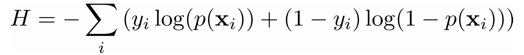
In a classification problem, the outputs 𝑦 are categorical, often either 0 or 1. For example, you might try to predict whether an email is spam or not. In the case of binary outputs, it’s convenient to minimize the cross-entropy function that also depends on the actual outputs 𝑦ᵢ and the corresponding predictions 𝑝(𝐱ᵢ):
In logistic regression, which is often used to solve classification problems, the functions 𝑝(𝐱) and 𝑓(𝐱) are defined as the following:
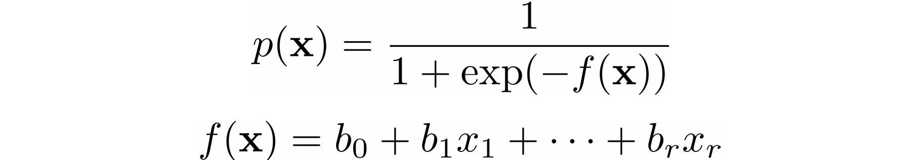
Again, you need to find the weights 𝑏₀, 𝑏₁, …, 𝑏ᵣ, but this time they should minimize the cross-entropy function.
Gradient of a Function: Calculus Refresher
In calculus, the derivative of a function shows you how much a value changes when you modify its argument (or arguments). Derivatives are important for optimization because the zero derivatives might indicate a minimum, maximum, or saddle point.
The gradient of a function 𝐶 of several independent variables 𝑣₁, …, 𝑣ᵣ is denoted with ∇𝐶(𝑣₁, …, 𝑣ᵣ) and defined as the vector function of the partial derivatives of 𝐶 with respect to each independent variable: ∇𝐶 = (∂𝐶/∂𝑣₁, …, ∂𝐶/𝑣ᵣ). The symbol ∇ is called nabla.
The nonzero value of the gradient of a function 𝐶 at a given point defines the direction and rate of the fastest increase of 𝐶. When working with gradient descent, you’re interested in the direction of the fastest decrease in the cost function. This direction is determined by the negative gradient, −∇𝐶.
Intuition Behind Gradient Descent
To understand the gradient descent algorithm, imagine a drop of water sliding down the side of a bowl or a ball rolling down a hill. The drop and the ball tend to move in the direction of the fastest decrease until they reach the bottom. With time, they’ll gain momentum and accelerate.
The idea behind gradient descent is similar: you start with an arbitrarily chosen position of the point or vector 𝐯 = (𝑣₁, …, 𝑣ᵣ) and move it iteratively in the direction of the fastest decrease of the cost function. As mentioned, this is the direction of the negative gradient vector, −∇𝐶.
Once you have a random starting point 𝐯 = (𝑣₁, …, 𝑣ᵣ), you update it, or move it to a new position in the direction of the negative gradient: 𝐯 → 𝐯 − 𝜂∇𝐶, where 𝜂 (pronounced “ee-tah”) is a small positive value called the learning rate.
The learning rate determines how large the update or moving step is. It’s a very important parameter. If 𝜂 is too small, then the algorithm might converge very slowly. Large 𝜂 values can also cause issues with convergence or make the algorithm divergent.
Implementation of Basic Gradient Descent
Now that you know how the basic gradient descent works, you can implement it in Python. You’ll use only plain Python and NumPy, which enables you to write concise code when working with arrays (or vectors) and gain a performance boost.
This is a basic implementation of the algorithm that starts with an arbitrary point, start, iteratively moves it toward the minimum, and returns a point that is hopefully at or near the minimum:
 1def gradient_descent(gradient, start, learn_rate, n_iter):
 2    vector = start
 3    for _ in range(n_iter):
 4        diff = -learn_rate * gradient(vector)
 5        vector += diff
 6    return vector
gradient_descent() takes four arguments:
gradientis the function or any Python callable object that takes a vector and returns the gradient of the function you’re trying to minimize.startis the point where the algorithm starts its search, given as a sequence (tuple, list, NumPy array, and so on) or scalar (in the case of a one-dimensional problem).learn_rateis the learning rate that controls the magnitude of the vector update.n_iteris the number of iterations.
This function does exactly what’s described above: it takes a starting point (line 2), iteratively updates it according to the learning rate and the value of the gradient (lines 3 to 5), and finally returns the last position found.
Before you apply gradient_descent(), you can add another termination criterion:
 1import numpy as np
 2
 3def gradient_descent(
 4    gradient, start, learn_rate, n_iter=50, tolerance=1e-06
 5):
 6    vector = start
 7    for _ in range(n_iter):
 8        diff = -learn_rate * gradient(vector)
 9        if np.all(np.abs(diff) <= tolerance):
10            break
11        vector += diff
12    return vector
You now have the additional parameter tolerance (line 4), which specifies the minimal allowed movement in each iteration. You’ve also defined the default values for tolerance and n_iter, so you don’t have to specify them each time you call gradient_descent().
Lines 9 and 10 enable gradient_descent() to stop iterating and return the result before n_iter is reached if the vector update in the current iteration is less than or equal to tolerance. This often happens near the minimum, where gradients are usually very small. Unfortunately, it can also happen near a local minimum or a saddle point.
Line 9 uses the convenient NumPy functions numpy.all() and numpy.abs() to compare the absolute values of diff and tolerance in a single statement. That’s why you import numpy on line 1.
Now that you have the first version of gradient_descent(), it’s time to test your function. You’ll start with a small example and find the minimum of the function 𝐶 = 𝑣².
This function has only one independent variable (𝑣), and its gradient is the derivative 2𝑣. It’s a differentiable convex function, and the analytical way to find its minimum is straightforward. However, in practice, analytical differentiation can be difficult or even impossible and is often approximated with numerical methods.
You need only one statement to test your gradient descent implementation:
>>> gradient_descent(
...     gradient=lambda v: 2 * v, start=10.0, learn_rate=0.2
... )
2.210739197207331e-06
You use the lambda function lambda v: 2 * v to provide the gradient of 𝑣². You start from the value 10.0 and set the learning rate to 0.2. You get a result that’s very close to zero, which is the correct minimum.
The figure below shows the movement of the solution through the iterations:
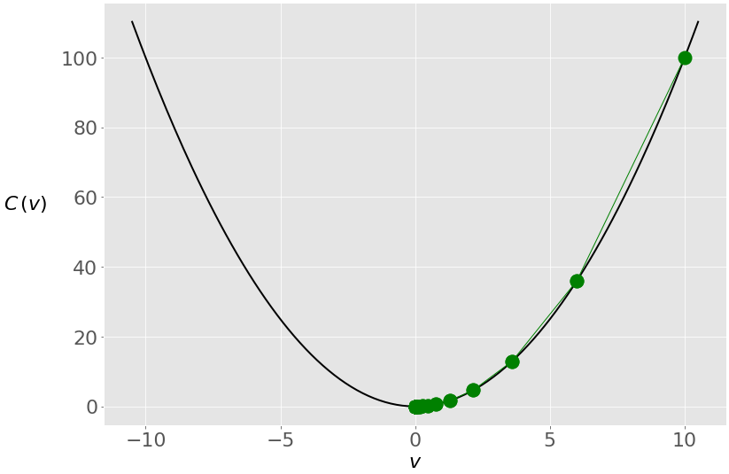
You start from the rightmost green dot (𝑣 = 10) and move toward the minimum (𝑣 = 0). The updates are larger at first because the value of the gradient (and slope) is higher. As you approach the minimum, they become lower.
Learning Rate Impact
The learning rate is a very important parameter of the algorithm. Different learning rate values can significantly affect the behavior of gradient descent. Consider the previous example, but with a learning rate of 0.8 instead of 0.2:
>>> gradient_descent(
...     gradient=lambda v: 2 * v, start=10.0, learn_rate=0.8
... )
-4.77519666596786e-07
You get another solution that’s very close to zero, but the internal behavior of the algorithm is different. This is what happens with the value of 𝑣 through the iterations:
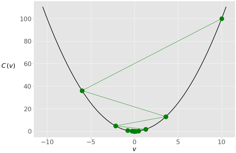
In this case, you again start with 𝑣 = 10, but because of the high learning rate, you get a large change in 𝑣 that passes to the other side of the optimum and becomes −6. It crosses zero a few more times before settling near it.
Small learning rates can result in very slow convergence. If the number of iterations is limited, then the algorithm may return before the minimum is found. Otherwise, the whole process might take an unacceptably large amount of time. To illustrate this, run gradient_descent() again, this time with a much smaller learning rate of 0.005:
>>> gradient_descent(
...     gradient=lambda v: 2 * v, start=10.0, learn_rate=0.005
... )
6.050060671375367
The result is now 6.05, which is nowhere near the true minimum of zero. This is because the changes in the vector are very small due to the small learning rate:

The search process starts at 𝑣 = 10 as before, but it can’t reach zero in fifty iterations. However, with a hundred iterations, the error will be much smaller, and with a thousand iterations, you’ll be very close to zero:
>>> gradient_descent(
...     gradient=lambda v: 2 * v, start=10.0, learn_rate=0.005,
...     n_iter=100
... )
3.660323412732294
>>> gradient_descent(
...     gradient=lambda v: 2 * v, start=10.0, learn_rate=0.005,
...     n_iter=1000
... )
0.0004317124741065828
>>> gradient_descent(
...     gradient=lambda v: 2 * v, start=10.0, learn_rate=0.005,
...     n_iter=2000
... )
9.952518849647663e-05
Nonconvex functions might have local minima or saddle points where the algorithm can get trapped. In such situations, your choice of learning rate or starting point can make the difference between finding a local minimum and finding the global minimum.
Consider the function 𝑣⁴ - 5𝑣² - 3𝑣. It has a global minimum in 𝑣 ≈ 1.7 and a local minimum in 𝑣 ≈ −1.42. The gradient of this function is 4𝑣³ − 10𝑣 − 3. Let’s see how gradient_descent() works here:
>>> gradient_descent(
...     gradient=lambda v: 4 * v**3 - 10 * v - 3, start=0,
...     learn_rate=0.2
... )
-1.4207567437458342
You started at zero this time, and the algorithm ended near the local minimum. Here’s what happened under the hood:
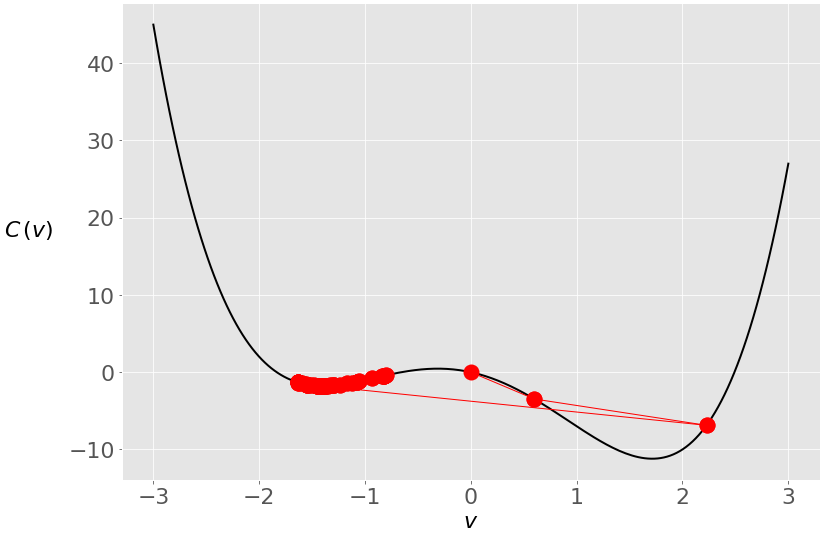
During the first two iterations, your vector was moving toward the global minimum, but then it crossed to the opposite side and stayed trapped in the local minimum. You can prevent this with a smaller learning rate:
>>> gradient_descent(
...     gradient=lambda v: 4 * v**3 - 10 * v - 3, start=0,
...     learn_rate=0.1
... )
1.285401330315467
When you decrease the learning rate from 0.2 to 0.1, you get a solution very close to the global minimum. Remember that gradient descent is an approximate method. This time, you avoid the jump to the other side:

A lower learning rate prevents the vector from making large jumps, and in this case, the vector remains closer to the global optimum.
Adjusting the learning rate is tricky. You can’t know the best value in advance. There are many techniques and heuristics that try to help with this. In addition, machine learning practitioners often tune the learning rate during model selection and evaluation.
Besides the learning rate, the starting point can affect the solution significantly, especially with nonconvex functions.
Application of the Gradient Descent Algorithm
In this section, you’ll see two short examples of using gradient descent. You’ll also learn that it can be used in real-life machine learning problems like linear regression. In the second case, you’ll need to modify the code of gradient_descent() because you need the data from the observations to calculate the gradient.
Short Examples
First, you’ll apply gradient_descent() to another one-dimensional problem. Take the function 𝑣 − log(𝑣). The gradient of this function is 1 − 1/𝑣. With this information, you can find its minimum:
>>> gradient_descent(
...     gradient=lambda v: 1 - 1 / v, start=2.5, learn_rate=0.5
... )
1.0000011077232125
With the provided set of arguments, gradient_descent() correctly calculates that this function has the minimum in 𝑣 = 1. You can try it with other values for the learning rate and starting point.
You can also use gradient_descent() with functions of more than one variable. The application is the same, but you need to provide the gradient and starting points as vectors or arrays. For example, you can find the minimum of the function 𝑣₁² + 𝑣₂⁴ that has the gradient vector (2𝑣₁, 4𝑣₂³):
>>> gradient_descent(
...     gradient=lambda v: np.array([2 * v[0], 4 * v[1]**3]),
...     start=np.array([1.0, 1.0]), learn_rate=0.2, tolerance=1e-08
... )
array([8.08281277e-12, 9.75207120e-02])
In this case, your gradient function returns an array, and the start value is an array, so you get an array as the result. The resulting values are almost equal to zero, so you can say that gradient_descent() correctly found that the minimum of this function is at 𝑣₁ = 𝑣₂ = 0.
Ordinary Least Squares
As you’ve already learned, linear regression and the ordinary least squares method start with the observed values of the inputs 𝐱 = (𝑥₁, …, 𝑥ᵣ) and outputs 𝑦. They define a linear function 𝑓(𝐱) = 𝑏₀ + 𝑏₁𝑥₁ + ⋯ + 𝑏ᵣ𝑥ᵣ, which is as close as possible to 𝑦.
This is an optimization problem. It finds the values of weights 𝑏₀, 𝑏₁, …, 𝑏ᵣ that minimize the sum of squared residuals SSR = Σᵢ(𝑦ᵢ − 𝑓(𝐱ᵢ))² or the mean squared error MSE = SSR / 𝑛. Here, 𝑛 is the total number of observations and 𝑖 = 1, …, 𝑛.
You can also use the cost function 𝐶 = SSR / (2𝑛), which is mathematically more convenient than SSR or MSE.
The most basic form of linear regression is simple linear regression. It has only one set of inputs 𝑥 and two weights: 𝑏₀ and 𝑏₁. The equation of the regression line is 𝑓(𝑥) = 𝑏₀ + 𝑏₁𝑥. Although the optimal values of 𝑏₀ and 𝑏₁ can be calculated analytically, you’ll use gradient descent to determine them.
First, you need calculus to find the gradient of the cost function 𝐶 = Σᵢ(𝑦ᵢ − 𝑏₀ − 𝑏₁𝑥ᵢ)² / (2𝑛). Since you have two decision variables, 𝑏₀ and 𝑏₁, the gradient ∇𝐶 is a vector with two components:
- ∂𝐶/∂𝑏₀ = (1/𝑛) Σᵢ(𝑏₀ + 𝑏₁𝑥ᵢ − 𝑦ᵢ) = mean(𝑏₀ + 𝑏₁𝑥ᵢ − 𝑦ᵢ)
- ∂𝐶/∂𝑏₁ = (1/𝑛) Σᵢ(𝑏₀ + 𝑏₁𝑥ᵢ − 𝑦ᵢ) 𝑥ᵢ = mean((𝑏₀ + 𝑏₁𝑥ᵢ − 𝑦ᵢ) 𝑥ᵢ)
You need the values of 𝑥 and 𝑦 to calculate the gradient of this cost function. Your gradient function will have as inputs not only 𝑏₀ and 𝑏₁ but also 𝑥 and 𝑦. This is how it might look:
def ssr_gradient(x, y, b):
    res = b[0] + b[1] * x - y
    return res.mean(), (res * x).mean()  # .mean() is a method of np.ndarray
ssr_gradient() takes the arrays x and y, which contain the observation inputs and outputs, and the array b that holds the current values of the decision variables 𝑏₀ and 𝑏₁. This function first calculates the array of the residuals for each observation (res) and then returns the pair of values of ∂𝐶/∂𝑏₀ and ∂𝐶/∂𝑏₁.
In this example, you can use the convenient NumPy method ndarray.mean() since you pass NumPy arrays as the arguments.
gradient_descent() needs two small adjustments:
- Add
xandyas the parameters ofgradient_descent()on line 4. - Provide
xandyto the gradient function and make sure you convert your gradient tuple to a NumPy array on line 8.
Here’s how gradient_descent() looks after these changes:
 1import numpy as np
 2
 3def gradient_descent(
 4    gradient, x, y, start, learn_rate=0.1, n_iter=50, tolerance=1e-06
 5):
 6    vector = start
 7    for _ in range(n_iter):
 8        diff = -learn_rate * np.array(gradient(x, y, vector))
 9        if np.all(np.abs(diff) <= tolerance):
10            break
11        vector += diff
12    return vector
gradient_descent() now accepts the observation inputs x and outputs y and can use them to calculate the gradient. Converting the output of gradient(x, y, vector) to a NumPy array enables elementwise multiplication of the gradient elements by the learning rate, which isn’t necessary in the case of a single-variable function.
Now apply your new version of gradient_descent() to find the regression line for some arbitrary values of x and y:
>>> x = np.array([5, 15, 25, 35, 45, 55])
>>> y = np.array([5, 20, 14, 32, 22, 38])

>>> gradient_descent(
...     ssr_gradient, x, y, start=[0.5, 0.5], learn_rate=0.0008,
...     n_iter=100_000
... )
array([5.62822349, 0.54012867])
The result is an array with two values that correspond to the decision variables: 𝑏₀ = 5.63 and 𝑏₁ = 0.54. The best regression line is 𝑓(𝑥) = 5.63 + 0.54𝑥. As in the previous examples, this result heavily depends on the learning rate. You might not get such a good result with too low or too high of a learning rate.
This example isn’t entirely random–it’s taken from the tutorial Linear Regression in Python. The good news is that you’ve obtained almost the same result as the linear regressor from scikit-learn. The data and regression results are visualized in the section Simple Linear Regression.
Improvement of the Code
You can make gradient_descent() more robust, comprehensive, and better-looking without modifying its core functionality:
 1import numpy as np
 2
 3def gradient_descent(
 4    gradient, x, y, start, learn_rate=0.1, n_iter=50, tolerance=1e-06,
 5    dtype="float64"
 6):
 7    # Checking if the gradient is callable
 8    if not callable(gradient):
 9        raise TypeError("'gradient' must be callable")
10
11    # Setting up the data type for NumPy arrays
12    dtype_ = np.dtype(dtype)
13
14    # Converting x and y to NumPy arrays
15    x, y = np.array(x, dtype=dtype_), np.array(y, dtype=dtype_)
16    if x.shape[0] != y.shape[0]:
17        raise ValueError("'x' and 'y' lengths do not match")
18
19    # Initializing the values of the variables
20    vector = np.array(start, dtype=dtype_)
21
22    # Setting up and checking the learning rate
23    learn_rate = np.array(learn_rate, dtype=dtype_)
24    if np.any(learn_rate <= 0):
25        raise ValueError("'learn_rate' must be greater than zero")
26
27    # Setting up and checking the maximal number of iterations
28    n_iter = int(n_iter)
29    if n_iter <= 0:
30        raise ValueError("'n_iter' must be greater than zero")
31
32    # Setting up and checking the tolerance
33    tolerance = np.array(tolerance, dtype=dtype_)
34    if np.any(tolerance <= 0):
35        raise ValueError("'tolerance' must be greater than zero")
36
37    # Performing the gradient descent loop
38    for _ in range(n_iter):
39        # Recalculating the difference
40        diff = -learn_rate * np.array(gradient(x, y, vector), dtype_)
41
42        # Checking if the absolute difference is small enough
43        if np.all(np.abs(diff) <= tolerance):
44            break
45
46        # Updating the values of the variables
47        vector += diff
48
49    return vector if vector.shape else vector.item()
gradient_descent() now accepts an additional dtype parameter that defines the data type of NumPy arrays inside the function. For more information about NumPy types, see the official documentation on data types.
In most applications, you won’t notice a difference between 32-bit and 64-bit floating-point numbers, but when you work with big datasets, this might significantly affect memory use and maybe even processing speed. For example, although NumPy uses 64-bit floats by default, TensorFlow often uses 32-bit decimal numbers.
In addition to considering data types, the code above introduces a few modifications related to type checking and ensuring the use of NumPy capabilities:
-
Lines 8 and 9 check if
gradientis a Python callable object and whether it can be used as a function. If not, then the function will raise aTypeError. -
Line 12 sets an instance of
numpy.dtype, which will be used as the data type for all arrays throughout the function. -
Line 15 takes the arguments
xandyand produces NumPy arrays with the desired data type. The argumentsxandycan be lists, tuples, arrays, or other sequences. -
Lines 16 and 17 compare the sizes of
xandy. This is useful because you want to be sure that both arrays have the same number of observations. If they don’t, then the function will raise aValueError. -
Line 20 converts the argument
startto a NumPy array. This is an interesting trick: ifstartis a Python scalar, then it’ll be transformed into a corresponding NumPy object (an array with one item and zero dimensions). If you pass a sequence, then it’ll become a regular NumPy array with the same number of elements. -
Line 23 does the same thing with the learning rate. This can be very useful because it enables you to specify different learning rates for each decision variable by passing a list, tuple, or NumPy array to
gradient_descent(). -
Lines 24 and 25 check if the learning rate value (or values for all variables) is greater than zero.
-
Lines 28 to 35 similarly set
n_iterandtoleranceand check that they are greater than zero. -
Lines 38 to 47 are almost the same as before. The only difference is the type of the gradient array on line 40.
-
Line 49 conveniently returns the resulting array if you have several decision variables or a Python scalar if you have a single variable.
Your gradient_descent() is now finished. Feel free to add some additional capabilities or polishing. The next step of this tutorial is to use what you’ve learned so far to implement the stochastic version of gradient descent.
Stochastic Gradient Descent Algorithms
Stochastic gradient descent algorithms are a modification of gradient descent. In stochastic gradient descent, you calculate the gradient using just a random small part of the observations instead of all of them. In some cases, this approach can reduce computation time.
Online stochastic gradient descent is a variant of stochastic gradient descent in which you estimate the gradient of the cost function for each observation and update the decision variables accordingly. This can help you find the global minimum, especially if the objective function is convex.
Batch stochastic gradient descent is somewhere between ordinary gradient descent and the online method. The gradients are calculated and the decision variables are updated iteratively with subsets of all observations, called minibatches. This variant is very popular for training neural networks.
You can imagine the online algorithm as a special kind of batch algorithm in which each minibatch has only one observation. Classical gradient descent is another special case in which there’s only one batch containing all observations.
Minibatches in Stochastic Gradient Descent
As in the case of the ordinary gradient descent, stochastic gradient descent starts with an initial vector of decision variables and updates it through several iterations. The difference between the two is in what happens inside the iterations:
- Stochastic gradient descent randomly divides the set of observations into minibatches.
- For each minibatch, the gradient is computed and the vector is moved.
- Once all minibatches are used, you say that the iteration, or epoch, is finished and start the next one.
This algorithm randomly selects observations for minibatches, so you need to simulate this random (or pseudorandom) behavior. You can do that with random number generation. Python has the built-in random module, and NumPy has its own random generator. The latter is more convenient when you work with arrays.
You’ll create a new function called sgd() that is very similar to gradient_descent() but uses randomly selected minibatches to move along the search space:
 1import numpy as np
 2
 3def sgd(
 4    gradient, x, y, start, learn_rate=0.1, batch_size=1, n_iter=50,
 5    tolerance=1e-06, dtype="float64", random_state=None
 6):
 7    # Checking if the gradient is callable
 8    if not callable(gradient):
 9        raise TypeError("'gradient' must be callable")
10
11    # Setting up the data type for NumPy arrays
12    dtype_ = np.dtype(dtype)
13
14    # Converting x and y to NumPy arrays
15    x, y = np.array(x, dtype=dtype_), np.array(y, dtype=dtype_)
16    n_obs = x.shape[0]
17    if n_obs != y.shape[0]:
18        raise ValueError("'x' and 'y' lengths do not match")
19    xy = np.c_[x.reshape(n_obs, -1), y.reshape(n_obs, 1)]
20
21    # Initializing the random number generator
22    seed = None if random_state is None else int(random_state)
23    rng = np.random.default_rng(seed=seed)
24
25    # Initializing the values of the variables
26    vector = np.array(start, dtype=dtype_)
27
28    # Setting up and checking the learning rate
29    learn_rate = np.array(learn_rate, dtype=dtype_)
30    if np.any(learn_rate <= 0):
31        raise ValueError("'learn_rate' must be greater than zero")
32
33    # Setting up and checking the size of minibatches
34    batch_size = int(batch_size)
35    if not 0 < batch_size <= n_obs:
36        raise ValueError(
37            "'batch_size' must be greater than zero and less than "
38            "or equal to the number of observations"
39        )
40
41    # Setting up and checking the maximal number of iterations
42    n_iter = int(n_iter)
43    if n_iter <= 0:
44        raise ValueError("'n_iter' must be greater than zero")
45
46    # Setting up and checking the tolerance
47    tolerance = np.array(tolerance, dtype=dtype_)
48    if np.any(tolerance <= 0):
49        raise ValueError("'tolerance' must be greater than zero")
50
51    # Performing the gradient descent loop
52    for _ in range(n_iter):
53        # Shuffle x and y
54        rng.shuffle(xy)
55
56        # Performing minibatch moves
57        for start in range(0, n_obs, batch_size):
58            stop = start + batch_size
59            x_batch, y_batch = xy[start:stop, :-1], xy[start:stop, -1:]
60
61            # Recalculating the difference
62            grad = np.array(gradient(x_batch, y_batch, vector), dtype_)
63            diff = -learn_rate * grad
64
65            # Checking if the absolute difference is small enough
66            if np.all(np.abs(diff) <= tolerance):
67                break
68
69            # Updating the values of the variables
70            vector += diff
71
72    return vector if vector.shape else vector.item()
You have a new parameter here. With batch_size, you specify the number of observations in each minibatch. This is an essential parameter for stochastic gradient descent that can significantly affect performance. Lines 34 to 39 ensure that batch_size is a positive integer no larger than the total number of observations.
Another new parameter is random_state. It defines the seed of the random number generator on line 22. The seed is used on line 23 as an argument to default_rng(), which creates an instance of Generator.
If you pass the argument None for random_state, then the random number generator will return different numbers each time it’s instantiated. If you want each instance of the generator to behave exactly the same way, then you need to specify seed. The easiest way is to provide an arbitrary integer.
Line 16 deduces the number of observations with x.shape[0]. If x is a one-dimensional array, then this is its size. If x has two dimensions, then .shape[0] is the number of rows.
On line 19, you use .reshape() to make sure that both x and y become two-dimensional arrays with n_obs rows and that y has exactly one column. numpy.c_[] conveniently concatenates the columns of x and y into a single array, xy. This is one way to make data suitable for random selection.
Finally, on lines 52 to 70, you implement the for loop for the stochastic gradient descent. It differs from gradient_descent(). On line 54, you use the random number generator and its method .shuffle() to shuffle the observations. This is one of the ways to choose minibatches randomly.
The inner for loop is repeated for each minibatch. The main difference from the ordinary gradient descent is that, on line 62, the gradient is calculated for the observations from a minibatch (x_batch and y_batch) instead of for all observations (x and y).
On line 59, x_batch becomes a part of xy that contains the rows of the current minibatch (from start to stop) and the columns that correspond to x. y_batch holds the same rows from xy but only the last column (the outputs). For more information about how indices work in NumPy, see the official documentation on indexing.
Now you can test your implementation of stochastic gradient descent:
>>> sgd(
...     ssr_gradient, x, y, start=[0.5, 0.5], learn_rate=0.0008,
...     batch_size=3, n_iter=100_000, random_state=0
... )
array([5.63093736, 0.53982921])
The result is almost the same as you got with gradient_descent(). If you omit random_state or use None, then you’ll get somewhat different results each time you run sgd() because the random number generator will shuffle xy differently.
Momentum in Stochastic Gradient Descent
As you’ve already seen, the learning rate can have a significant impact on the result of gradient descent. You can use several different strategies for adapting the learning rate during the algorithm execution. You can also apply momentum to your algorithm.
You can use momentum to correct the effect of the learning rate. The idea is to remember the previous update of the vector and apply it when calculating the next one. You don’t move the vector exactly in the direction of the negative gradient, but you also tend to keep the direction and magnitude from the previous move.
The parameter called the decay rate or decay factor defines how strong the contribution of the previous update is. To include the momentum and the decay rate, you can modify sgd() by adding the parameter decay_rate and use it to calculate the direction and magnitude of the vector update (diff):
 1import numpy as np
 2
 3def sgd(
 4    gradient, x, y, start, learn_rate=0.1, decay_rate=0.0, batch_size=1,
 5    n_iter=50, tolerance=1e-06, dtype="float64", random_state=None
 6):
 7    # Checking if the gradient is callable
 8    if not callable(gradient):
 9        raise TypeError("'gradient' must be callable")
10
11    # Setting up the data type for NumPy arrays
12    dtype_ = np.dtype(dtype)
13
14    # Converting x and y to NumPy arrays
15    x, y = np.array(x, dtype=dtype_), np.array(y, dtype=dtype_)
16    n_obs = x.shape[0]
17    if n_obs != y.shape[0]:
18        raise ValueError("'x' and 'y' lengths do not match")
19    xy = np.c_[x.reshape(n_obs, -1), y.reshape(n_obs, 1)]
20
21    # Initializing the random number generator
22    seed = None if random_state is None else int(random_state)
23    rng = np.random.default_rng(seed=seed)
24
25    # Initializing the values of the variables
26    vector = np.array(start, dtype=dtype_)
27
28    # Setting up and checking the learning rate
29    learn_rate = np.array(learn_rate, dtype=dtype_)
30    if np.any(learn_rate <= 0):
31        raise ValueError("'learn_rate' must be greater than zero")
32
33    # Setting up and checking the decay rate
34    decay_rate = np.array(decay_rate, dtype=dtype_)
35    if np.any(decay_rate < 0) or np.any(decay_rate > 1):
36        raise ValueError("'decay_rate' must be between zero and one")
37
38    # Setting up and checking the size of minibatches
39    batch_size = int(batch_size)
40    if not 0 < batch_size <= n_obs:
41        raise ValueError(
42            "'batch_size' must be greater than zero and less than "
43            "or equal to the number of observations"
44        )
45
46    # Setting up and checking the maximal number of iterations
47    n_iter = int(n_iter)
48    if n_iter <= 0:
49        raise ValueError("'n_iter' must be greater than zero")
50
51    # Setting up and checking the tolerance
52    tolerance = np.array(tolerance, dtype=dtype_)
53    if np.any(tolerance <= 0):
54        raise ValueError("'tolerance' must be greater than zero")
55
56    # Setting the difference to zero for the first iteration
57    diff = 0
58
59    # Performing the gradient descent loop
60    for _ in range(n_iter):
61        # Shuffle x and y
62        rng.shuffle(xy)
63
64        # Performing minibatch moves
65        for start in range(0, n_obs, batch_size):
66            stop = start + batch_size
67            x_batch, y_batch = xy[start:stop, :-1], xy[start:stop, -1:]
68
69            # Recalculating the difference
70            grad = np.array(gradient(x_batch, y_batch, vector), dtype_)
71            diff = decay_rate * diff - learn_rate * grad
72
73            # Checking if the absolute difference is small enough
74            if np.all(np.abs(diff) <= tolerance):
75                break
76
77            # Updating the values of the variables
78            vector += diff
79
80    return vector if vector.shape else vector.item()
In this implementation, you add the decay_rate parameter on line 4, convert it to a NumPy array of the desired type on line 34, and check if it’s between zero and one on lines 35 and 36. On line 57, you initialize diff before the iterations start to ensure that it’s available in the first iteration.
The most important change happens on line 71. You recalculate diff with the learning rate and gradient but also add the product of the decay rate and the old value of diff. Now diff has two components:
decay_rate * diffis the momentum, or impact of the previous move.-learn_rate * gradis the impact of the current gradient.
The decay and learning rates serve as the weights that define the contributions of the two.
Random Start Values
As opposed to ordinary gradient descent, the starting point is often not so important for stochastic gradient descent. It may also be an unnecessary difficulty for a user, especially when you have many decision variables. To get an idea, just imagine if you needed to manually initialize the values for a neural network with thousands of biases and weights!
In practice, you can start with some small arbitrary values. You’ll use the random number generator to get them:
 1import numpy as np
 2
 3def sgd(
 4    gradient, x, y, n_vars=None, start=None, learn_rate=0.1,
 5    decay_rate=0.0, batch_size=1, n_iter=50, tolerance=1e-06,
 6    dtype="float64", random_state=None
 7):
 8    # Checking if the gradient is callable
 9    if not callable(gradient):
10        raise TypeError("'gradient' must be callable")
11
12    # Setting up the data type for NumPy arrays
13    dtype_ = np.dtype(dtype)
14
15    # Converting x and y to NumPy arrays
16    x, y = np.array(x, dtype=dtype_), np.array(y, dtype=dtype_)
17    n_obs = x.shape[0]
18    if n_obs != y.shape[0]:
19        raise ValueError("'x' and 'y' lengths do not match")
20    xy = np.c_[x.reshape(n_obs, -1), y.reshape(n_obs, 1)]
21
22    # Initializing the random number generator
23    seed = None if random_state is None else int(random_state)
24    rng = np.random.default_rng(seed=seed)
25
26    # Initializing the values of the variables
27    vector = (
28        rng.normal(size=int(n_vars)).astype(dtype_)
29        if start is None else
30        np.array(start, dtype=dtype_)
31    )
32
33    # Setting up and checking the learning rate
34    learn_rate = np.array(learn_rate, dtype=dtype_)
35    if np.any(learn_rate <= 0):
36        raise ValueError("'learn_rate' must be greater than zero")
37
38    # Setting up and checking the decay rate
39    decay_rate = np.array(decay_rate, dtype=dtype_)
40    if np.any(decay_rate < 0) or np.any(decay_rate > 1):
41        raise ValueError("'decay_rate' must be between zero and one")
42
43    # Setting up and checking the size of minibatches
44    batch_size = int(batch_size)
45    if not 0 < batch_size <= n_obs:
46        raise ValueError(
47            "'batch_size' must be greater than zero and less than "
48            "or equal to the number of observations"
49        )
50
51    # Setting up and checking the maximal number of iterations
52    n_iter = int(n_iter)
53    if n_iter <= 0:
54        raise ValueError("'n_iter' must be greater than zero")
55
56    # Setting up and checking the tolerance
57    tolerance = np.array(tolerance, dtype=dtype_)
58    if np.any(tolerance <= 0):
59        raise ValueError("'tolerance' must be greater than zero")
60
61    # Setting the difference to zero for the first iteration
62    diff = 0
63
64    # Performing the gradient descent loop
65    for _ in range(n_iter):
66        # Shuffle x and y
67        rng.shuffle(xy)
68
69        # Performing minibatch moves
70        for start in range(0, n_obs, batch_size):
71            stop = start + batch_size
72            x_batch, y_batch = xy[start:stop, :-1], xy[start:stop, -1:]
73
74            # Recalculating the difference
75            grad = np.array(gradient(x_batch, y_batch, vector), dtype_)
76            diff = decay_rate * diff - learn_rate * grad
77
78            # Checking if the absolute difference is small enough
79            if np.all(np.abs(diff) <= tolerance):
80                break
81
82            # Updating the values of the variables
83            vector += diff
84
85    return vector if vector.shape else vector.item()
You now have the new parameter n_vars that defines the number of decision variables in your problem. The parameter start is optional and has the default value None. Lines 27 to 31 initialize the starting values of the decision variables:
- If you provide a
startvalue other thanNone, then it’s used for the starting values. - If
startisNone, then your random number generator creates the starting values using the standard normal distribution and the NumPy method.normal().
Now give sgd() a try:
>>> sgd(
...     ssr_gradient, x, y, n_vars=2, learn_rate=0.0001,
...     decay_rate=0.8, batch_size=3, n_iter=100_000, random_state=0
... )
array([5.63014443, 0.53901017])
You get similar results again.
You’ve learned how to write the functions that implement gradient descent and stochastic gradient descent. The code above can be made more robust and polished. You can also find different implementations of these methods in well-known machine learning libraries.
Gradient Descent in Keras and TensorFlow
Stochastic gradient descent is widely used to train neural networks. The libraries for neural networks often have different variants of optimization algorithms based on stochastic gradient descent, such as:
- Adam
- Adagrad
- Adadelta
- RMSProp
These optimization libraries are usually called internally when neural network software is trained. However, you can use them independently as well:
>>> import tensorflow as tf

>>> # Create needed objects
>>> sgd = tf.keras.optimizers.SGD(learning_rate=0.1, momentum=0.9)
>>> var = tf.Variable(2.5)
>>> cost = lambda: 2 + var ** 2

>>> # Perform optimization
>>> for _ in range(100):
...     sgd.minimize(cost, var_list=[var])

>>> # Extract results
>>> var.numpy()
-0.007128528
>>> cost().numpy()
2.0000508
In this example, you first import tensorflow and then create the object needed for optimization:
sgdis an instance of the stochastic gradient descent optimizer with a learning rate of0.1and a momentum of0.9.varis an instance of the decision variable with an initial value of2.5.costis the cost function, which is a square function in this case.
The main part of the code is a for loop that iteratively calls .minimize() and modifies var and cost. Once the loop is exhausted, you can get the values of the decision variable and the cost function with .numpy().
You can find more information on these algorithms in the Keras and TensorFlow documentation. The article An overview of gradient descent optimization algorithms offers a comprehensive list with explanations of gradient descent variants.
Conclusion
You now know what gradient descent and stochastic gradient descent algorithms are and how they work. They’re widely used in the applications of artificial neural networks and are implemented in popular libraries like Keras and TensorFlow.
In this tutorial, you’ve learned:
- How to write your own functions for gradient descent and stochastic gradient descent
- How to apply your functions to solve optimization problems
- What the key features and concepts of gradient descent are, like learning rate or momentum, as well as its limitations
You’ve used gradient descent and stochastic gradient descent to find the minima of several functions and to fit the regression line in a linear regression problem. You’ve also seen how to apply the class SGD from TensorFlow that’s used to train neural networks.
If you have questions or comments, then please put them in the comment section below.


