Emulating Quantum Computing with Python

In this blog: Learn the principles of quantum computing using Python. Download our “Quantum Computing” environment to get a version of Python 3.8 and the QuTiP framework explained in this post.

Google’s recent proclamation of quantum supremacy (whether true or not) showed that quantum computing is moving from theory to practice at an accelerating rate. While most computers on the planet today are still reliant on standard silicon processors, Moore’s Law (the trend of doubling the number of transistors in an integrated circuit every two years) is approaching its physical limitation, opening the way for a new model.

The simple fact is that as transistors get smaller and smaller, approaching the size of a few atoms, the classical physics that governs their behavior is superseded by quantum mechanics. This has brought about a whole new set of engineering and design challenges that have given rise to the quantum computer.

While quantum computers can be used for everything a classical computer can do (including a quantum computing version of Minecraft), the way they work is fundamentally different. Unfortunately, access to a quantum computer remains rare. For those interested in seeing for themselves how they work, the best way is to simulate quantum computing with classical computers.

The Quantum Toolbox in Python, or QuTiP for short, provides one such platform for simulating the dynamics of open quantum systems. One of the most common problems in quantum information processing is the presence of noise in the system. This noise is typically due to interaction between the quantum bits, or qubits, and the surrounding physical system. Understanding how this noise influences the outcome of computations is essential to understanding (and designing) well-behaved quantum computers.

In this article, I’ll use Python and QuTiP to simulate this noise in order to understand how it influences a model qubit system. While understanding the complexities of quantum mechanics is challenging, platforms such as QuTiP provide an alternative, practical approach to learning quantum physics for those who are not physicists. Don’t worry if you have never taken a course in quantum mechanics, as a basic knowledge of Python is all that is necessary to understand the code in this article!

Installing Python for Quantum Computing

To follow along with the code in this article, you’ll need to have a recent version of Python, the QuTiP package, and all of its dependencies. The easiest way to set up a Python environment with everything you need is to download and install our pre-built “Quantum Computing” environment, which contains a version of Python 3.8 and the QuTiP package used in this post.

Just follow these two steps:

1. Install the ActiveState Platform’s CLI, the State Tool on Windows using Powershell:

   IEX(New-Object Net.WebClient).downloadString('https://platform.activestate.com/dl/cli/install.ps1')

   Or install the State Tool on Linux:

   sh <(curl -q https://platform.activestate.com/dl/cli/install.sh)

2. Run the following command to download the environment and automatically install it into a virtual environment:

   state activate Pizza-Team/quantum-computing
   

All of the code used in this article can be found on my GitLab repository.  All set? Let’s go.

Qubit Basics

At the heart of quantum information processing lies coherent state control. In classical computing, a bit can either be in a 0 or 1 state. In quantum computing, a qubit can either be in a 0 state, a 1 state, or a superposition state of both 0 and 1. 

This superposition state is achieved by applying a pulse (mathematically equivalent to a rotation operation), or a series of pulses. Because the pulse is an interaction between the qubit and the surrounding system, it generates noise. The quality of the pulse then plays a role in determining how well the superposition state is achieved.

With QuTiP, we can create a model qubit system, and then apply control pulses with and without noise to quantify how the magnitude of noise influences the fidelity of the superposition state. In practice, physicists can determine how much noise is present in the pulse, but not how well the superposition state is prepared. This is why tools like QuTiP are helpful.        

Defining a Qubit & Control Pulse in Python

In QuTiP, we simulate rotations on an N qubit system using the Processor class. We are considering only a single qubit, so N = 1 in our case. To add control pulses, we use the add_control method. I add two pulses: σ_z and σ_y. These have deeper meaning in terms of quantum mechanics, but it is sufficient to know that executing these pulses in series is how to prepare the qubit in the superposition state:

processor = Processor(N=1)
processor.add_control(0.5 * sigmaz(), targets=0, label="sigmaz")
processor.add_control(0.5 * sigmay(), targets=0, label="sigmay")

To see the characteristics of each pulse, we can run:

for pulse in processor.pulses:
    pulse.print_info()

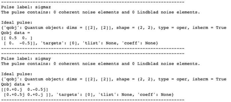
The pulse σ_z in matrix representation is given under Qobj data. The target corresponds to the target qubit, which the pulse interacts with. We only have one, so the default Python labeling is 0. tlist and coeff correspond to the pulse time sequence and strength, respectively. We can use a Numpy array to define both:

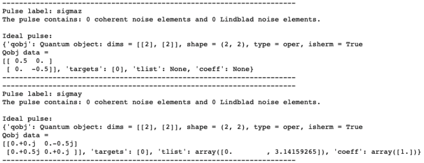
processor.pulses[1].coeff = np.array([1.]) # pulse strength set to 1
processor.pulses[1].tlist = np.array([0., pi]) #time sequence defined from 0 to pi
for pulse in processor.pulses:
    pulse.print_info()

These definitions correspond to a σ_y pulse for t=π and with strength 1. Notice the difference in the output:

To observe the effect of the σ_y pulse on the qubit, first we need to initialize the qubit state. I initialize it in the 0 state:

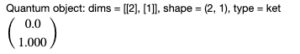
To observe t#define initial state
basis0 = basis(2, 0)
basis0

Output:

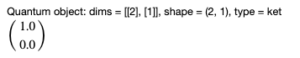
The way to mathematically represent the 0 state is a 2×1 matrix with the first row set to 1. The 1 state is represented by a 1 in the second row. To run the simulation:

result = processor.run_state(init_state=basis0)
result.states[-1].tidyup(1.0e-5)

Output:

The qubit is now in the 1 state! For those readers experienced in linear algebra or quantum physics this is not surprising, since the pulse we applied is a π rotation around the y-axis on a Bloch sphere. Now, to prepare the qubit into the superposition state, I’ll implement a series of three pulses:

#rotations to prepare superposition state
processor.pulses[0].coeff = np.array([1., 0., 1.])
processor.pulses[1].coeff = np.array([0., 1., 0.])
processor.pulses[0].tlist = np.array([0., pi/2., 2*pi/2, 3*pi/2])
processor.pulses[1].tlist = np.array([0., pi/2., 2*pi/2, 3*pi/2])

The initial state is 1 (because of the previous pulse we applied). After running the following:

result = processor.run_state(init_state=basis(2, 1))
result.states[-1].tidyup(1e-5)

The results are:

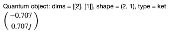
This matrix represents the superposition state composed of both the 0 and 1 state. To visualize the change of states of the qubit after each pulse on a Bloch sphere:

b = Bloch()
b.add_states(result.states)
b.make_sphere()

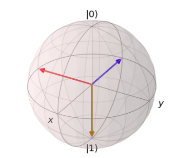
The initial state is 1, which corresponds to a vector pointing in the -z direction. After the first pulse, the qubit maintains the same state (yellow vector). The blue and red vectors correspond to the qubit state after the second and third pulse. In this geometric representation, the xy-plane corresponds to a superposition state with a 50% probability amplitude of observing a 0 or a 1 state. For performing quantum computations, any deviations from this 50-50 split are not ideal (i.e. geometrically, vectors that do not lie on the xy-plane). 

To add noise, I’ll initialize two separate qubits and define the same pulse strengths and time sequence for each:

processor = Processor(N=1)
processor.add_control(0.5 * sigmaz(), targets=0, label="sigmaz")
processor.add_control(0.5 * sigmay(), targets=0, label="sigmay")
processor.coeffs = np.array([[1., 0., 1.],
                             [0., 1., 0.]])
processor.set_all_tlist(np.array([0., pi/2., 2*pi/2, 3*pi/2]))
#create copy and add noise to coeff array
processor_white = copy.deepcopy(processor)
processor_white.add_noise(RandomNoise(rand_gen=np.random.normal, dt=0.1, loc=-0.05, scale=0.5))

In the above code, I’ve added random noise to the coeff values of the second qubit. The following code initializes each in the 1 state:

result = processor.run_state(init_state=basis(2, 1))
result.states[-1].tidyup(1.0e-5)

Output:

As expected, the code results in the same result as we obtained previously for the case of a pulse with no noise. Now let’s try a noisy pulse:

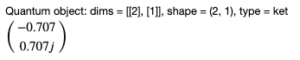
result_white = processor_white.run_state(init_state=basis(2, 1))
result_white.states[-1].tidyup(1.0e-4)

Output:

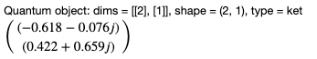
Note the difference in the matrix values. To quantify the overlap between the two states, we can use the fidelity function:

fidelity(result.states[-1], result_white.states[-1])

Output:

0.935514109499076

Or to compare the two graphically:

b = Bloch()
b.add_states([result.states[-1], result_white.states[-1]])
b.make_sphere()

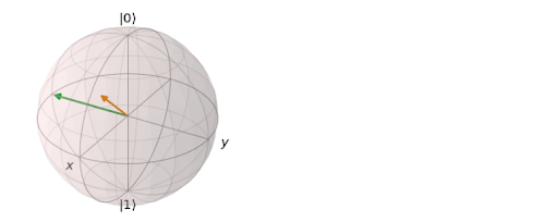
The green vector corresponds to the state with no noise, while the orange vector corresponds to the state with noise. Notice that it is no longer in the xy-plane. To further investigate the effect of the noise, feel free to play with the scale factor in the RandomNoise function.

Summary

In this article, I used Python’s QuTiP package to simulate the effect of noise within the control pulse when preparing a qubit into the superposition state. This is a common problem plaguing quantum computing, and needs to be better understood and controlled for before quantum computers can become mainstream. Tools such as Python, that rely on classical computation techniques, are instrumental in making progress towards this end.

• All of the code used in this article can be found on my GitLab repository.
• Sign up for a free ActiveState Platform account so you can download the pre-built Quantum Computing environment and start learning more about quantum computing in Python.  

 

 

Related Blogs:

The Top 10 Python Frameworks for Web Development

Top 10 Python Packages Every Developer Should Learn