Introducing constrained optimization through two simple examples

Optimization is all around us. Various physical entities are constantly solving some form of optimization problem: water running downhill (finding state of least energy), light rays trying traveling between two points (finding route of shortest time), or electric currents finding paths of least resistance. Optimization is also used extensively in industry. In explicit forms, it is used to maximize or minimize quantities of interest (portfolio returns, supply chains). In implicit forms, optimization algorithms are the backbone of machine learning and curve-fitting algorithms.

One great way to build intuition for optimization algorithms is to pick a simple problem and solve it numerically using the algorithm of choice. A ‘simple problem’ can be any problem whose solution is known or can be readily guessed. Since we don’t have to think about the answer, we can use such problems to understand how the algorithm arrives at the answer, building valuable intuition in the process.

Given their omnipresence, there is a large pool of simple optimization problems for us to choose for our exploration. We want a problem whose answer we can guess but which also includes all essential elements of a real optimization problem. One such simple-but-rich problem for exploring constrained optimization is the isoperimetric problem:

Among all closed curves of fixed perimeter, which curve maximizes the area of its enclosed region?

In other words, given a closed loop of an inelastic thread, the problem asks us to find the shape that maximizes the enclosed area. In an earlier post we showed that the answer is a circle. Here we will demonstrate this answer numerically.

Here is our plan for this post. We will start by stating the optimization problem in an abstract mathematical form. We will then show step-by-step how the math translates to code. For some algorithms, we will use existing libraries, others we will code from scratch. For brevity, we will show only the important snippets of code, the full code can be found in our Github.

Abstract problem statement

Let us start by stating the problem mathematically. Assume that the desired shape is planar and is represented as a function $y = f(x)$. Let $A(y)$ be the area of this shape and $S(y)$ be its perimeter. In a sense, $y$ is our shorthand for writing ‘any shape’ and $A(y)$ and $S(y)$ denote area and perimeter of ‘that shape’. In this notation, the problem statement is:

Translating abstract problem into code

For a numerical solution, we need to a way to represent concepts like ‘any shape’ in code and provide a way to compute its area and perimeter.

Representing a shape

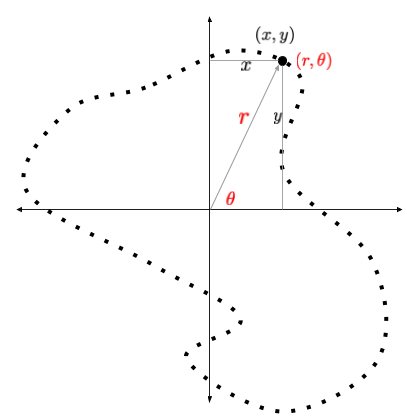
One way to represent a shape is as a list of two dimensional points. Each point in the list is either a pair of its $x$ and $y$ coordinates or a tuple of $r$ and $\theta$ coordinates. Both representations are equivalent and are shown in the figure below. We’ll need both representations for our solution. It is simple to translate an $(r, \theta)$ point to an $(x, y)$ point and below we will include a utility function pol2cart() to do just that.

Ok so we have a list of points, but how can we ensure that this list represents a shape and not just a random cloud of points? For points to be on a shape, we need to be able to go to the next or the previous point from the current one. This property is called ordering. Without the ability to tell adjacent points, we cant compute the perimeter. After all, perimeter is precisely the sum of distances between adjacent points.

A simple way to get an ordered list of random points on a plane is to loop through angles between $0$ through $360^\circ$ and assign a random radius to each point, as shown in the code below.

def generate_points(n_points):
    theta = np.linspace(-np.pi, np.pi, n_points)
    radius = np.random.uniform(0.5, 1.5, size=(n_points,))
    return radius, theta

The above function returns the list of points in the polar $(r, \theta)$ coordinates. We can convert them into cartesian $(x, y)$ coordinates using a convenience function:

def pol2cart(r, theta):
    x = r * np.cos(theta)
    y = r * np.sin(theta)
    return x, y

When plotted, our starting shape looks like this:

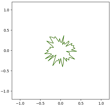
Now we can represent and generate an arbitrary planar shape. Next we need to compute its perimeter and the area.

Computing the area and the perimeter

The get the area and perimeter computing code, our starting point is the formulas from introductory calculus:

We’re giving both versions because the area turns out to be easier to compute in $(r, \theta)$ and the perimeter in $(x, y)$.

Computing the area

Roughly, the integral sign is simply a shorthand for a for loop. Therefore an implementation for the area formula in $(r, \theta)$ coordinates is:

# r = list of radii, theta = list of theta values
def area(r, theta):
    dtheta = theta[1] - theta[0]
    A = 0.0
    for i in range(len(r)):
        A += 0.5 * r[i] * r[i] * dtheta
    return A

We can get a faster implementation using numerical integration routines such as the Simpsons rule. With the use of ready-made Scipy function, our area computation code is particularly simple:

from scipy.integrate import simps
def area(r, theta):
    return 0.5 * simps(r * r, theta)

Computing the perimeter

This perimeter expression is more complicated because it involves derivative. Fortunately, since we have a table of ordered $(x, y)$ values, we can avoid derivatives and directly obtain the perimeter by summing distances between consecutive points:

The above equation says to loop over the list index and add up the Pythagorean distance between consecutive points:

def perimeter(x, y):
    """
    x = list of x-coordinates
    y = list of y-coordinates
    """
    S = 0.0
    for i in range(len(x) - 1):
        S += sqrt((x[i+1] - x[i]) ** 2  + (y[i+1] - y[i]) ** 2)
    return S

A more efficient (but equivalent) implementation uses Numpy:

def perimeter(x, y):
    dx = np.diff(x)
    dy = np.diff(y)
    return np.sqrt((dx * dx + dy * dy)).sum()

The optimization objective

With the implementation of area and perimeter in hand, we’re ready to take the final step in the problem specification. To modify our initial loop to enclose maximum area, we need to modify each point in the list so that the loop occupies more and more area. However, we want to increase the area while keeping the perimeter fixed. To build in this constraint, we will construct a function that depends on both the area and the perimeter. The minimum value of this function will give us a list of points that simultaneously maximises the area and pins the perimeter. That function is the following:

The function $L$ is called variously as the loss function, cost function, objective function or the Lagrangian. The claim is that if we find a list of points $(r, \theta)$ that minimizes the function $L$ without constraints, then it is the same as having solved our problem of maximizing the area with the perimeter constraint.

Lets convince ourselves why. The function $L$ will be minimized when $-A$ is minimized (i.e. $A$ is maximized) and the difference between computed perimeters and $C$ is $0$. A list $r$ of radius values that maximizes $A$ and minimizes deviation between $A$ and $C$ is exactly what we’re after. So if we get such a list, then it means we’ve solved the problem.

def loss(r, theta, C, lambda1):
    A = area(r, theta)
    S = perimeter(r, theta)
    L = -A + lambda1 * (S - C) ** 2
    return L

Notice that loss() uses the area() and the perimeter() functions that we just implemented.

The implementation of the loss() function completes the specification of the problem. Next step is to find the list of $r$ values that yields the minimum value of loss. We will do this minimization using the following algorithms:

• Greedy algorithm, coded from scratch
• Adam optimizer in Pytorch
• Stochastic gradient descent in Pytorch
• Gradient descent, coded from scratch

The algorithms listed above belong to a class called iterative algorithms. Each starts from an initial guess and, in each step, modifies the solution to come up with a improved solution. This part is common to all. The difference is in how each improves the current solution.

Lastly, it is important to note that the solution found by an algorithm may be right or wrong. When a wrong solution is found, we usually tweak the parameters and rerun. In one examples below, we’ll see an example of an algorithm converging but to a wrong solution.

Greedy algorithm

In each iteration, the greedy algorithm modifies the shape slightly by adding a small random value to the coordinates of a randomly selected point. This modification can make the $L$ function better or worse. If the $L$ function is better, we accept the change. Otherwise we dont. The code is more or less a direct translation of the description:

def greedy(r, theta, C, lambda1, n_iterations):
    n_points = r.shape[0]
    best_r = r.copy()
    best_loss = loss(best_r, theta, C, lambda1)

    for i in range(n_iterations):
        old_r = r.copy()
        j = np.random.randint(0, n_points)
        r[j] += np.random.uniform(-0.01, 0.01)
        new_loss = loss(r, theta, C, lambda1)

        if new_loss < best_loss:
            best_loss = new_loss
            best_r = r
        else:
            r = old_r

    return best_r, theta

Following animation shows the convergence behavior of the first $10^5$ iterations of the greedy algorithm. The greedy algorithm recovers the circular shape to a reasonable accuracy.

Adam and SGD (Pytorch)

Next we will use Adam and SGD (stochastic gradient descent) optimizers in Pytorch. Instead of randomly modifying the shape, these optimizers inspect the function to look for the downward slope and change the list of points according to that. Moreover many (or all) elements of the $r$ list are changed at once, instead of just one. Both these modifications speed up the convergence significantly. Further details of Adam and SGD are out of scope for this post. However, we will go through the process of casting our problem in the language of neural network, which allows us to use any available optimizer in a library like Pytorch.

A typical problem solved with neural nets is supervised: we have a list of input-output pairs: Image/labels, audio/words, or sentence/sentiment and we seek to minimize the prediction error. The isoperimetric problem, on the other hand, is a pure optimization problem. We aren’t provided any input/output pairs. Our problem is to arrange $N$ ordered points into a shape that maximizes the area formed by their loop while keeping the perimeter fixed. Therefore our input will be a constant and output will be a list of radius values (one for each value of $\theta$ between $0^\circ$ and $360^\circ$).

Though we have no inputs, we still need parameters whose adjustments will give us the list of points. These adjustable parameters are called ‘weights’ in neural network language. To begin, we create our fully-connected 1-layer network architecture with 1 input, 100 hidden weights and $N$ outputs.

The Pytorch code to create the network is below:

class Inet(nn.Module):
    def __init__(self, n_in, n_hidden, n_out):
        super(Inet, self).__init__()
        self.main = nn.Sequential(
            nn.Linear(n_in, n_hidden, bias=False),
            nn.Tanh(),
            nn.Linear(n_hidden, n_out, bias=False)
        )

    def forward(self, input_):
        return self.main(input_)

To define the loss function for the network, we need a re-implementation of the area() and the perimeter() in terms of (differentiable) Pytorch functions. The difference from the Numpy version is that we replace Numpy ndarray with Pytorch tensors.

def perimeter(x, y):
    dx = x[1:] - x[:-1]
    dy = y[1:] - y[:-1]
    return torch.sqrt((dx*dx + dy * dy)).sum()

def area(r, theta):
    return 0.5 * torch.trapz(r * r, theta)

The work up to here is common for all optimizer algorithms. To choose a particular optimization algorithms we simply create an instance of the appropriate optimizer as shown below. Finally, we instantiate our neural net, and iterate till convergence:

def nnet_optimizer(r, theta, learning_rate, lambda1, algorithm):
    num_points = r.shape[0]
    theta = torch.tensor(theta)
    r = torch.tensor(r)
    model = Inet(1, 100, num_points)
    if algorithm == 'adam':
        optimizer = torch.optim.Adam(model.parameters(), lr=learning_rate)
    else:
        optimizer = torch.optim.SGD(model.parameters(), lr=learning_rate, momentum=0.9)

    input = torch.tensor([1.])
    for i in range(n_iterations):
        r = model(input)
        L = loss(r, theta, lambda1, lambda2)
        optimizer.zero_grad()
        L.backward()
        optimizer.step()

    return r, theta

The animation below shows successful convergence of the Adam optimizer to the right solution.

However, Adam often finds wrong solution as seen below. These wrong solutions are called ‘local minimums’, which means kind of a bad quality solution to the problem.

Below is the result of SGD optimizer with learning rate of $10^{-4}$ and momentum of $0.5$. Without momentum, the SGD failed to converge in our implementation.

Here is another run of SGD with a stronger momentum term of $0.9$. The convergence is faster but less stable than the previous version.

Hand-coded gradient descent

The final algorithm we’ll use is gradient descent, derived and coded from scratch. Recall that any iterative algorithm needs to update the inputs in order to get a better value for $L$ function. The greedy algorithm didn’t use any information about the problem; it modified the input randomly. This randomness is why it took $10^5$ steps to converge. Gradient descent will tell us how much adjustment to make, and it will converge in $5000$ steps.

Since we will be deriving the gradient descent equations, there will be more math here than in the previous sections. The basic gradient descent update rule is

In words, the above rule tells us the amount of update to the $i$th element of the $r$ list is equal to a small number $\alpha$ times the derivative of $L$ with respect to that $i$th element. Lets unpack the meaning of this equation further.

We saw before that the objective function $L$ is a function of $r$ list: i.e a function of each element $r_i$ (or, if you prefer, r[i]) of the list. We can express this explicitly as $L(r) = L(r_1, r_2, \ldots, r_N)$. The update rule instructs us to compute the update to the $i$th element in the following way: (1) differentiate the $L$ function with respect to each $r_i$, (2) evaluate the numerical value of the derivative, and lastly (3) multiply that value by a small number. This is the amount by which we should update the $i$th element. When we carry out the procedure for all $N$ elements, we have a better list.

To compute the derivatives by hand, we need a a modified version of our cost function that is equivalent to the previous one but expresses the perimeter in terms of $r$:

This directly gives us the required derivatives.

We have one such equation for each $i = 1,\ldots,N$. We could try to code this complicated looking expression and it is possible that we may get a correct answer. But lets observe the two terms more carefully. The first term is strongly dependent on $r_i$. The second term is not only weakly dependent, but its influence on the update rule diminishes the closer we get to the correct answer. This is because when we’re in the vicinity of the answer, the computed perimeter is close to the constraint value, so $S(r) - C \approx 0$. Because of the different relative strengths of the two terms we make a small (mathematically unjustified) adjustment to the derivative; we ignore the square root term and get the following simplified expression:

With this simplification we can write our gradient descent update rule explicitly as

The code translation for this equation looks is straightforward:

def gradient_descent(r, theta, C, learning_rate, lambda1):
    d_theta = theta[1] - theta[0]
    for i in range(n_iterations):
        S = perimeter(r, theta)
        dL_dr = -d_theta * r + 2.0 * lambda1 * d_theta * (S - C)
        r -= learning_rate * dL_dr
    return r, theta

The following animation shows how our hand-coded gradient descent algorithm converges to its optimal shape. The convergence is more uniform compared to the greedy algorithm. It is also faster ($\sim 5000$ steps).

Bonus: The Max Entropy Problem

To consolidate our understanding of the steps, we will solve another cool problem, the max entropy problem. This problem originates from probability theory and one of its statement reads:

Among all probability distributions $p(x)$ of known mean $\mu$ and known variance $\sigma^2$ find the one with largest entropy.

Entropy of a probability distribution is a measure of information provided by the samples of random variables drawn from it. So the max entropy problem can also be specified as: among all possible probability distributions having mean $\mu$ and variance $\sigma^2$, find the shape of the one with maximum information. In an earlier post we saw that this shape is the normal (Gaussian) distribution.

This time we will go through the steps quicker than before. However, each section here parallels the one for the isoperimetric problem. You’re encouraged to pause and review our description from the isoperimetric problem if needed.

Mathematical expressions for the various quantities in the problem are as follows. As before, we will provide code for each of the expressions.

With these definitions, the max entropy problem can be expressed as

Previously we showed theoretically that the solution to the max entropy problem is a normal distribution centered at $\mu$ with a standard deviation $\sigma$. Here we will see an optimization algorithm numerically converge to the normal distribution. This problem is a bit more complex than the isoperimetric problem because of more constraints. The procedure, however, remains the same: we express the problem in a single $L$ function using use the method of Lagrange multipliers:

The interpretation of this equation is simple: we seek a list of probability values $p_i$ for each $x_i$ such that the entropy $H(p)$ is maximized while keeping the mean, the standard deviation, the normalization values fixed. This will be achieved when we find a list of $p$ values which minimize $-H(p)$ and each of the square terms are close to $0$. Therefore a list of $p_i$ values that minimizes $L(p)$ will solve our problem.

To code this, we need implementation of the loss function, which in turn requires code for the entropy, mean, the standard deviation, and the normalization functions. We have already seen how to use numerical integration (Simpsons rule) to implement functions involving integrals:

def entropy(x, y):
    return simps(-y * np.log(y), x)

def mean(x, y):
    return simps(x * y, x)

def stddev(x, y):
    mu = mean(x, y)
    var = simps(x * x * y, x) - mu * mu
    return np.sqrt(var)

def norm(x, y):
    return simps(y, x)

def loss(x, y, mu, sigma, lambda1, lambda2, lambda3):
    H = entropy(x, y)
    M = mean(x, y)
    S = stddev(x, y)
    N = norm(x, y)
    L = -H + lambda1 * (M - mu) ** 2 \
           + lambda2 * (S - sigma) ** 2 \
           + lambda3 * (N - 1.0) ** 2
    return L

The next step is to minimize the loss function using the optimization algorithms we have used earlier in the article: greedy, Pytorch-SGD and hand-coded gradient descent. The implementation of the greedy and the Pytorch methods is similar to the way we did it for the isoperimetric problem. We wont reproduce the code below, but it can be found in our Github repository. We will, however, derive the expressions for the hand-coded gradient descent since it provides useful intuition for the descent methods.

We start by initializing $128$ equally-spaced $x$ values in $(-5, 5)$. For each $x_i$ we pick a $p_i$ from a uniform random distribution. To make things interesting let us fix the mean and the standard deviation to $\mu = 1$ and $\sigma = 0.5$. We then demand list of $p_i$ values that will maximize the entropy and whose mean is $\mu$, standard deviation is $\sigma$ and whose normalization is $1$.

Greedy algorithm

The animation below shows $100$ equally spaced frames from the first $10^5$ iterations of the greedy algorithm run on a list of $128$ points. We can see that the greedy algorithm converges to a Gaussian with mean $1$ and standard deviation $0.52$.

Hand-coded gradient descent

To implement gradient descent from scratch, we will need as before to dig through the math. We start with with discretizing the equations (i.e. replacing the integrals with summations) and obtain an expression for $\frac{\partial L}{\partial p_i}$ and plug that into the gradient descent update rule. We have done this process before.

The discrete version of the $L$ is obtained by discretizing the entropy, mean, standard deviation, and the normalization.

From these equations we can derive the gradient term

and input into the gradient descent optimizer:

def gradient_descent(x, y, mu0, sigma0, lambda1, lambda2, lambda3,
                    learning_rate,  n_iterations):
    dx = x[1] - x[0]
    epsy = 1e-12
    for i in range(n_iterations):
        N = norm(x, y)
        M = mean(x, y)
        S = stddev(x, y)
        dL_dp = (1 + np.log(y)) \
                 + 2. * lambda1 * x * (M - mu0) \
                 + lambda2 * x * x * (1 - sigma0 / S) \
                 + 2. * lambda3 * (N - 1.)

        y -= learning_rate * dx * grad_L
        y = np.clip(y, epsy, None)
    return x, y

The animation below shows our hand-coded gradient descent optimization routine converging nicely to the expected normal distribution.

Pytorch SGD

Finally we will use the SGD optimizer in Pytorch to solve this problem. As before we need to translate the code for loss computation from Numpy to Pytorch. Because these changes are nominal, we will not reproduce the code here and instead refer the reader to our Github.

The animation below shows our best results with the Pytorch SGD optimizer. We user a learning rate of $10^{-4}$ and a momentum of $0.5$.

A few things to note about the SGD optimizer. Even after extensively tuning the learning parameters, we found it difficult to get the SGD to converge with a small number of points. We had to use more than $4000$ points to get the converged result to resemble a normal distribution. Even then, the standard deviation of the converged result is $0.82$ instead of the expected $0.5$ (off by over $50\%$). Adam optimizer gave us similar experience. The greedy and the hand-coded gradient descent converged accurately to the expected parameters. I’m investigating the convergence issue and will update if a solution is found.

Summary and exercises

We saw numerical solution of two classic optimization problems using a few different algorithms. We went through the exercise of translating an abstract problem into Python code. We then coded the greedy and gradient descent algorithms from scratch to solve the problem. Finally we generated the animations of their convergence. Complete code for all of the above steps is available on our Github. Below are a couple of suggested exercises if you want to try your hand at solving some similar problems.

• Set up an optimization problem to show that the shortest distance between two points is a straight line and solve it using greedy algorithm, hand-coded gradient descent and Pytorch.

• Set up and numerically solve the Brachistochrone problem.