
Machine learning and data science come with a set of problems that are different from what you’ll find in traditional software engineering. Version control systems help developers manage changes to source code. But data version control, managing changes to models and datasets, isn’t so well established.
It’s not easy to keep track of all the data you use for experiments and the models you produce. Accurately reproducing experiments that you or others have done is a challenge. Many teams are actively developing tools and frameworks to solve these problems.
In this tutorial, you’ll learn how to:
- Use a tool called DVC to tackle some of these challenges
- Track and version your datasets and models
- Share a single development computer between teammates
- Create reproducible machine learning experiments
This tutorial includes several examples of data version control techniques in action. To follow along, you can get the repository with the sample code by clicking the following link:
Get the Source Code: Click here to get the source code you’ll use to learn about data version control with DVC in this tutorial.
What Is Data Version Control?
In standard software engineering, many people need to work on a shared codebase and handle multiple versions of the same code. This can quickly lead to confusion and costly mistakes.
To address this problem, developers use version control systems, such as Git, that help keep team members organized.
In a version control system, there’s a central repository of code that represents the current, official state of the project. A developer can make a copy of that project, make some changes, and request that their new version become the official one. Their code is then reviewed and tested before it’s deployed to production.
These quick feedback cycles can happen many times per day in traditional development projects. But similar conventions and standards are largely missing from commercial data science and machine learning. Data version control is a set of tools and processes that tries to adapt the version control process to the data world.
Having systems in place that allow people to work quickly and pick up where others have left off would increase the speed and quality of delivered results. It would enable people to manage data transparently, run experiments effectively, and collaborate with others.
Note: An experiment in this context means either training a model or running operations on a dataset to learn something from it.
One tool that helps researchers govern their data and models and run reproducible experiments is DVC, which stands for Data Version Control.
What Is DVC?
DVC is a command-line tool written in Python. It mimics Git commands and workflows to ensure that users can quickly incorporate it into their regular Git practice. If you haven’t worked with Git before, then be sure to check out Introduction to Git and GitHub for Python Developers. If you’re familiar with Git but would like to take your skills to the next level, then check out Advanced Git Tips for Python Developers.
DVC is meant to be run alongside Git. In fact, the git and dvc commands will often be used in tandem, one after the other. While Git is used to store and version code, DVC does the same for data and model files.
Git can store code locally and also on a hosting service like GitHub, Bitbucket, or GitLab. Likewise, DVC uses a remote repository to store all your data and models. This is the single source of truth, and it can be shared amongst the whole team. You can get a local copy of the remote repository, modify the files, then upload your changes to share with team members.
The remote repository can be on the same computer you’re working on, or it can be in the cloud. DVC supports most major cloud providers, including AWS, GCP, and Azure. But you can set up a DVC remote repository on any server and connect it to your laptop. There are safeguards to keep members from corrupting or deleting the remote data.
When you store your data and models in the remote repository, a .dvc file is created. A .dvc file is a small text file that points to your actual data files in remote storage.
The .dvc file is lightweight and meant to be stored with your code in GitHub. When you download a Git repository, you also get the .dvc files. You can then use those files to get the data associated with that repository. Large data and model files go in your DVC remote storage, and small .dvc files that point to your data go in GitHub.
The best way to understand DVC is to use it, so let’s dive in. You’ll explore the most important features by working through several examples. Before you start, you’ll need to set up an environment to work in and then get some data.
Set Up Your Working Environment
In this tutorial, you’ll learn how to use DVC by practicing on examples that work with image data. You’ll play around with lots of image files and train a machine learning model that recognizes what an image contains.
To work through the examples, you’ll need to have Python and Git installed on your system. You can follow the Python 3 Installation and Setup Guide to install Python on your system. To install Git, you can read through Installing Git.
Since DVC is a command-line tool, you’ll need to be familiar with working in your operating system’s command line. If you’re a Windows user, have a look at Running DVC on Windows.
To prepare your workspace, you’ll take the following steps:
- Create and activate a virtual environment.
- Install DVC and its prerequisite Python libraries.
- Fork and clone a GitHub repository with all the code.
- Download a free dataset to use in the examples.
You can use any package and environment manager you want. This tutorial uses conda because it has great support for data science and machine learning tools. To create and activate a virtual environment, open your command-line interface of choice and type the following command:
$ conda create --name dvc python=3.8.2 -y
The create command creates a new virtual environment. The --name switch gives a name to that environment, which in this case is dvc. The python argument allows you to select the version of Python that you want installed inside the environment. Finally, the -y switch automatically agrees to install all the necessary packages that Python needs, without you having to respond to any prompts.
Once everything is installed, activate the environment:
$ conda activate dvc
You now have a Python environment that is separate from your operating system’s Python installation. This gives you a clean slate and prevents you from accidentally messing up something in your default version of Python.
You’ll also use some external libraries in this tutorial:
dvcis the star of this tutorial.scikit-learnis a machine learning library that allows you to train models.scikit-imageis an image processing library that you’ll use to prepare data for training.pandasis a library for data analysis that organizes data in table-like structures.numpyis a numerical computing library that adds support for multidimensional data, like images.
Some of these are available only through conda-forge, so you’ll need to add it to your config and use conda install to install all the libraries:
$ conda config --add channels conda-forge
$ conda install dvc scikit-learn scikit-image pandas numpy
Alternatively, you can use the pip installer:
$ python -m pip install dvc scikit-learn scikit-image pandas numpy
Now you have all the necessary Python libraries to run the code.
This tutorial comes with a ready-to-go repository that contains the directory structure and code to quickly get you experimenting with DVC. You can get the repository by clicking on the link below:
Get the Source Code: Click here to get the source code you’ll use to learn about data version control with DVC in this tutorial.
You need to fork the repository to your own GitHub account. On the repository’s GitHub page, click Fork in the top-right corner of the screen and select your private account in the window that pops up. GitHub will create a forked copy of the repository under your account.
Clone the forked repository to your computer with the git clone command and position your command line inside the repository folder:
$ git clone https://github.com/YourUsername/data-version-control
$ cd data-version-control
Don’t forget to replace YourUsername in the above command with your actual username. You should now have a clone of the repository on your computer.
Here’s the folder structure for the repository:
data-version-control/
|
├── data/
│   ├── prepared/
│   └── raw/
|
├── metrics/
├── model/
└── src/
    ├── evaluate.py
    ├── prepare.py
    └── train.py
There are six folders in your repository:
src/is for source code.data/is for all versions of the dataset.data/raw/is for data obtained from an external source.data/prepared/is for data modified internally.model/is for machine learning models.data/metrics/is for tracking the performance metrics of your models.
The src/ folder contains three Python files:
prepare.pycontains code for preparing data for training.train.pycontains code for training a machine learning model.evaluate.pycontains code for evaluating the results of a machine learning model.
The final step in the preparation is to get an example dataset you can use to practice DVC. Images are well suited for this particular tutorial because managing lots of large files is where DVC shines, so you’ll get a good look at DVC’s most powerful features. You’ll use the Imagenette dataset from fastai.
Imagenette is a subset of the ImageNet dataset, which is often used as a benchmark dataset in many machine learning papers. ImageNet is too big to use as an example on a laptop, so you’ll use the smaller Imagenette dataset. Go to the Imagenette GitHub page and click 160 px download in the README.
This will download the dataset compressed into a TAR archive. Mac users can extract the files by double-clicking the archive in the Finder. Linux users can unpack it with the tar command. Windows users will need to install a tool that unpacks TAR files, like 7-zip.
The dataset is structured in a particular way. It has two main folders:
train/includes images used for training a model.val/includes images used for validating a model.
Note: Validation usually happens while the model is training so researchers can quickly understand how well the model is doing. Since this tutorial isn’t focused on performance metrics, you’ll use the validation set for testing your model after it’s been trained.
Imagenette is a classification dataset, which means each image has an associated class that describes what’s in the image. To solve a classification problem, you need to train a model that can accurately determine the class of an image. It needs to look at an image and correctly identify what’s being shown.
The train/ and val/ folders are further divided into multiple folders. Each folder has a code that represents one of the 10 possible classes, and each image in this dataset belongs to one of ten classes:
- Tench
- English springer
- Cassette player
- Chain saw
- Church
- French horn
- Garbage truck
- Gas pump
- Golf ball
- Parachute
For simplicity and speed, you’ll train a model using only two of the ten classes, golf ball and parachute. When trained, the model will accept any image and tell you whether it’s an image of a golf ball or an image of a parachute. This kind of problem, in which a model decides between two kinds of objects, is called binary classification.
Copy the train/ and val/ folders and put them into your new repository, in the data/raw/ folder. Your repository structure should now look like this:
data-version-control/
|
├── data/
│   ├── prepared/
│   └── raw/
│       ├── train/
│       │   ├── n01440764/
│       │   ├── n02102040/
│       │   ├── n02979186/
│       │   ├── n03000684/
│       │   ├── n03028079/
│       │   ├── n03394916/
│       │   ├── n03417042/
│       │   ├── n03425413/
│       │   ├── n03445777/
│       │   └── n03888257/
|       |
│       └── val/
│           ├── n01440764/
│           ├── n02102040/
│           ├── n02979186/
│           ├── n03000684/
│           ├── n03028079/
│           ├── n03394916/
│           ├── n03417042/
│           ├── n03425413/
│           ├── n03445777/
│           └── n03888257/
|
├── metrics/
├── model/
└── src/
    ├── evaluate.py
    ├── prepare.py
    └── train.py
Alternatively, you can get the data using the curl command:
$ curl https://s3.amazonaws.com/fast-ai-imageclas/imagenette2-160.tgz \
    -O imagenette2-160.tgz
The backslash (\) allows you to separate a command into multiple rows for better readability. The above command will download the TAR archive.
You can then extract the dataset and move it to the data folders:
$ tar -xzvf imagenette2-160.tgz
$ mv imagenette2-160/train data/raw/train
$ mv imagenette2-160/val data/raw/val
Finally, remove the archive and the extracted folder:
$ rm -rf imagenette2-160
$ rm imagenette2-160.tgz
Great! You’ve completed the setup and are ready to start playing with DVC.
Practice the Basic DVC Workflow
The dataset you downloaded is enough to start practicing the DVC basics. In this section, you’ll see how DVC works in tandem with Git to manage your code and data.
To start, create a branch for your first experiment:
$ git checkout -b "first_experiment"
git checkout changes your current branch, and the -b switch tells Git that this branch doesn’t exist and should be created.
Next, you need to initialize DVC. Make sure you’re positioned in the top-level folder of the repository, then run dvc init:
$ dvc init
This will create a .dvc folder that holds configuration information, just like the .git folder for Git. In principle, you don’t ever need to open that folder, but you’ll take a peek in this tutorial so you can understand what’s happening under the hood.
Note: DVC has recently started collecting anonymized usage analytics so the authors can better understand how DVC is used. This helps them improve the tool. You can turn it off by setting the analytics configuration option to false:
$ dvc config core.analytics false
Git gives you the ability to push your local code to a remote repository so that you have a single source of truth shared with other developers. Other people can check out your code and work on it locally without fear of corrupting the code for everyone else. The same is true for DVC.
You need some kind of remote storage for the data and model files controlled by DVC. This can be as simple as another folder on your system. Create a folder somewhere on your system outside the data-version-control/ repository and call it dvc_remote.
Now come back to your data-version-control/ repository and tell DVC where the remote storage is on your system:
$ dvc remote add -d remote_storage path/to/your/dvc_remote
DVC now knows where to back up your data and models. dvc remote add stores the location to your remote storage and names it remote_storage. You can choose another name if you want. The -d switch tells DVC that this is your default remote storage. You can add more than one storage location and switch between them.
You can always check what your repository’s remote is. Inside the .dvc folder of your repository is a file called config, which stores configuration information about the repository:
[core]
    analytics = false
    remote = remote_storage
['remote "remote_storage"']
    url = /path/to/your/remote_storage
remote = remote_storage sets your remote_storage folder as the default, and ['remote "remote_storage"'] defines the configuration of your remote. The url points to the folder on your system. If your remote storage were a cloud storage system instead, then the url variable would be set to a web URL.
DVC supports many cloud-based storage systems, such as AWS S3 buckets, Google Cloud Storage, and Microsoft Azure Blob Storage. You can find out more in the official DVC documentation for the dvc remote add command.
Your repository is now initialized and ready for work. You’ll cover three basic actions:
- Tracking files
- Uploading files
- Downloading files
The basic rule of thumb you’ll follow is that small files go to GitHub, and large files go to DVC remote storage.
Tracking Files
Both Git and DVC use the add command to start tracking files. This puts the files under their respective control.
Add the train/ and val/ folders to DVC control:
$ dvc add data/raw/train
$ dvc add data/raw/val
Images are considered large files, especially if they’re collected into datasets with hundreds or thousands of files. The add command adds these two folders under DVC control. Here’s what DVC does under the hood:
- Adds your
train/andval/folders to.gitignore - Creates two files with the
.dvcextension,train.dvcandval.dvc - Copies the
train/andval/folders to a staging area
This process is a bit complex and warrants a more detailed explanation.
.gitignore is a text file that has a list of files that Git should ignore, or not track. When a file is listed in .gitignore, it’s invisible to git commands. By adding the train/ and val/ folders to .gitignore, DVC makes sure you won’t accidentally upload large data files to GitHub.
You learned about .dvc files in the section What is DVC? They’re small text files that point DVC to your data in remote storage. Remember the rule of thumb: large data files and folders go into DVC remote storage, but the small .dvc files go into GitHub. When you come back to your work and check out all the code from GitHub, you’ll also get the .dvc files, which you can use to get your large data files.
Finally, DVC copies the data files to a staging area. The staging area is called a cache. When you initialized DVC with dvc init, it created a .dvc folder in your repository. In that folder, it created the cache folder, .dvc/cache. When you run dvc add, all the files are copied to .dvc/cache.
This raises two questions:
- Doesn’t copying files waste a lot of space?
- Can you put the cache somewhere else?
The answer to both questions is yes. You’ll work through both of these issues in the section Share a Development Machine.
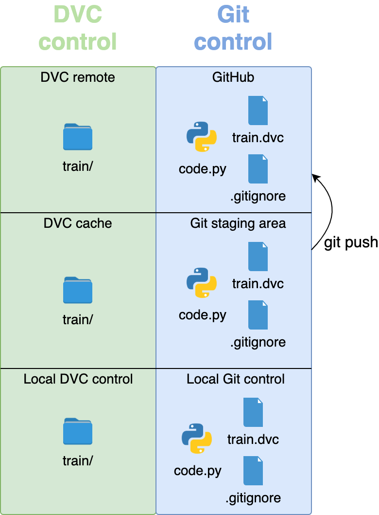
Here’s what the repository looks like before any commands are executed:
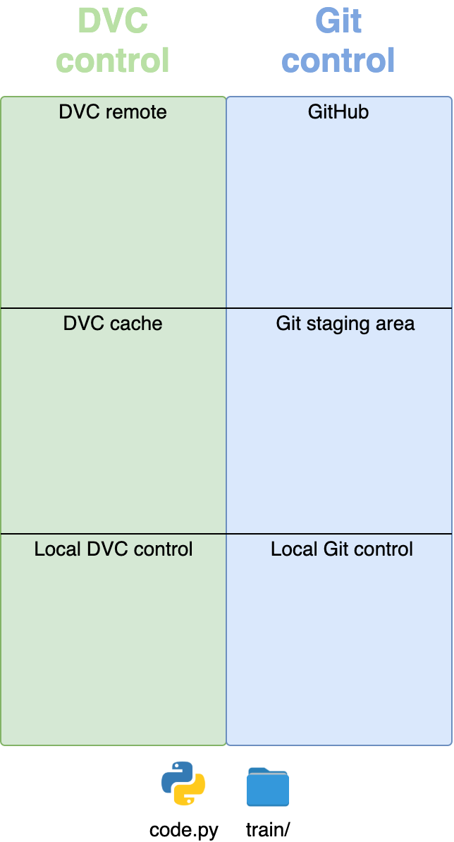
Everything that DVC controls is on the left (in green) and everything that Git controls is on the right (in blue). The local repository has a code.py file with Python code and a train/ folder with training data. This is a simplified version of what will happen with your repository.
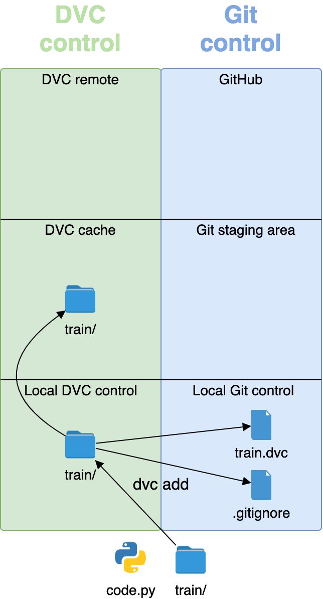
When you run dvc add train/, the folder with large files goes under DVC control, and the small .dvc and .gitignore files go under Git control. The train/ folder also goes into the staging area, or cache:
Once the large image files have been put under DVC control, you can add all the code and small files to Git control with git add:
$ git add --all
The --all switch adds all files that are visible to Git to the staging area.
Now all the files are under the control of their respective version control systems:
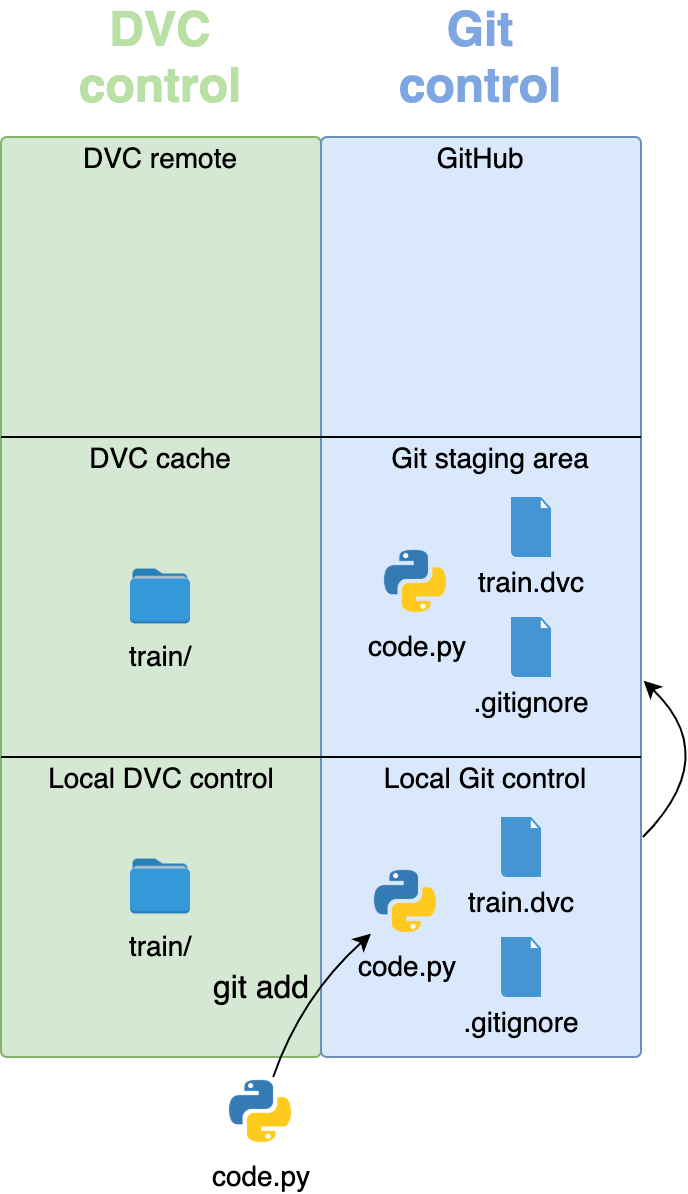
To recap, large image files go under DVC control, and small files go under Git control. If someone wants to work on your project and use the train/ and val/ data, then they would first need to download your Git repository. They could then use the .dvc files to get the data.
But before people can get your repository and data, you need to upload your files to remote storage.
Uploading Files
To upload files to GitHub, you first need to create a snapshot of the current state of your repository. When you add all the modified files to the staging area with git add, create a snapshot with the commit command:
$ git commit -m "First commit with setup and DVC files"
The -m switch means the quoted text that follows is a commit message explaining what was done. This command turns individual tracked changes into a full snapshot of the state of your repository.
DVC also has a commit command, but it doesn’t do the same thing as git commit. DVC doesn’t need a snapshot of the whole repository. It can just upload individual files as soon as they’re tracked with dvc add.
You use dvc commit when an already tracked file changes. If you make a local change to the data, then you would commit the change to the cache before uploading it to remote. You haven’t changed your data since it was added, so you can skip the commit step.
Note: Since this part of DVC is different from Git, you might want to read more about the add and commit commands in the official DVC documentation.
To upload your files from the cache to the remote, use the push command:
$ dvc push
DVC will look through all your repository folders to find .dvc files. As mentioned, these files will tell DVC what data needs to be backed up, and DVC will copy them from the cache to remote storage:
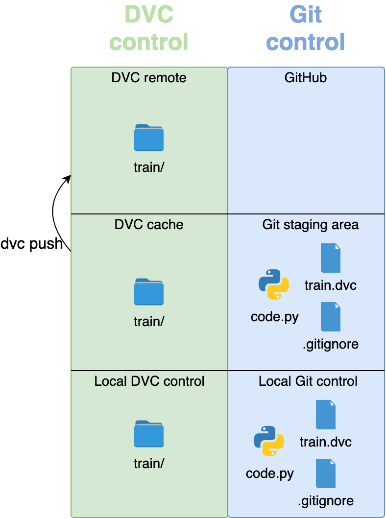
Your data is now safely stored in a location away from your repository. Finally, push the files under Git control to GitHub:
$ git push --set-upstream origin first_experiment
GitHub doesn’t know about the new branch you created locally, so the first push needs to use the --set-upstream option. origin is the place where your main, hosted version of the code is. In this case, it means GitHub. Your code and other small files are now safely stored in GitHub:
Well done! All your files have been backed up in remote storage.
Downloading Files
To learn how to download files, you first need to remove some of them from your repository.
As soon as you’ve added your data with dvc add and pushed it with dvc push, it’s backed up and safe. If you want to save space, you can remove the actual data. As long as all the files are tracked by DVC, and their .dvc files are in your repository, you can quickly get the data back.
You can remove the entire val/ folder, but make sure that the .dvc file doesn’t get removed:
$ rm -rf data/raw/val
This will delete the data/raw/val/ folder from your repository, but the folder is still safely stored in your cache and the remote storage. You can get it back at any time.
To get your data back from the cache, use the dvc checkout command:
$ dvc checkout data/raw/val.dvc
Your data/raw/val/ folder has been restored. If you want DVC to search through your whole repository and check out everything that’s missing, then use dvc checkout with no additional arguments.
When you clone your GitHub repository on a new machine, the cache will be empty. The fetch command gets the contents of the remote storage into the cache:
$ dvc fetch data/raw/val.dvc
Or you can use just dvc fetch to get the data for all DVC files in the repository. Once the data is in your cache, check it out to the repository with dvc checkout. You can perform both fetch and checkout with a single command, dvc pull:
$ dvc pull
dvc pull executes dvc fetch followed by dvc checkout. It copies your data from the remote to the cache and into your repository in a single sweep. These commands roughly mimic what Git does, since Git also has fetch, checkout, and pull commands:
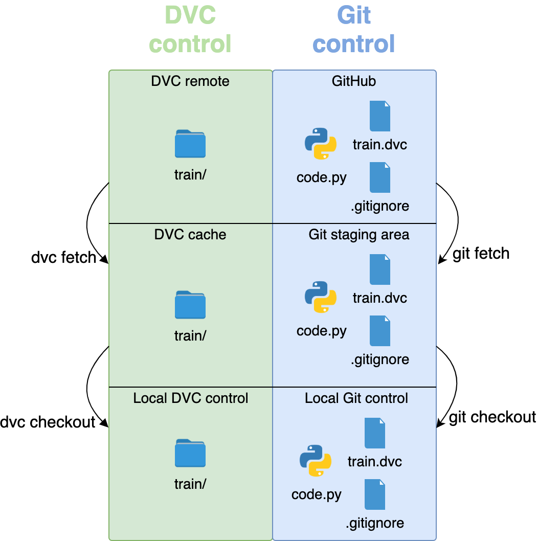
Keep in mind that you first need to get the .dvc files from Git, and only then can you call DVC commands like fetch and checkout to get your data. If the .dvc files aren’t in your repository, then DVC won’t know what data you want to fetch and check out.
You’ve now learned the basic workflow for DVC and Git. Whenever you add more data or change some code, you can add, commit, and push to keep everything versioned and safely backed up. For many people, this basic workflow will be enough for their everyday needs.
The rest of this tutorial focuses on some specific use cases like sharing computers with multiple people and creating reproducible pipelines. To explore how DVC handles these problems, you’ll need to have some code that runs machine learning experiments.
Build a Machine Learning Model
Using the Imagenette dataset, you’ll train a model to distinguish between images of golf balls and parachutes.
You’ll follow three main steps:
- Prepare data for training.
- Train your machine learning model.
- Evaluate the performance of your model.
As mentioned before, these steps correspond with the three Python files in the src/ folder:
prepare.pytrain.pyevaluate.py
The following subsections will explain what each file does. The entire file contents will be shown, followed by an explanation of what each line does.
Preparing Data
Since the data is stored in multiple folders, Python would need to search through all of them to find the images. The folder name determines what the label is. This might not be difficult for a computer, but it’s not very intuitive for a human.
To make the data easier to use, you’ll create a CSV file that will contain a list of all images and their labels to use for training. The CSV file will have two columns, a filename column containing the full path for a single image, and a label column that will contain the actual label string, like "golf ball" or "parachute". Each row will represent one image.
This is a sneak peek of what the CSV will look like:
filename, label
full/path/to/data-version-control/raw/n03445777/n03445777_5768.JPEG,golf ball
full/path/to/data-version-control/raw/n03445777/n03445777_5768,golf ball
full/path/to/data-version-control/raw/n03445777/n03445777_11967.JPEG,golf ball
...
You’ll need two CSV files:
train.csvwill contain a list of images for training.test.csvwill contain a list of images for testing.
You can create the CSV files by running the prepare.py script, which has three main steps:
- Map folder names like
n03445777/to label names likegolf ball. - Get a list of files for the
golf ballandparachutelabels. - Save the
filelist-labelpairs as a CSV file.
Here’s the source code you’ll use for the preparation step:
 1# prepare.py
 2from pathlib import Path
 3
 4import pandas as pd
 5
 6FOLDERS_TO_LABELS = {
 7    "n03445777": "golf ball",
 8    "n03888257": "parachute"
 9    }
10
11def get_files_and_labels(source_path):
12    images = []
13    labels = []
14    for image_path in source_path.rglob("*/*.JPEG"):
15        filename = image_path.absolute()
16        folder = image_path.parent.name
17        if folder in FOLDERS_TO_LABELS:
18            images.append(filename)
19            label = FOLDERS_TO_LABELS[folder]
20            labels.append(label)
21    return images, labels
22
23def save_as_csv(filenames, labels, destination):
24    data_dictionary = {"filename": filenames, "label": labels}
25    data_frame = pd.DataFrame(data_dictionary)
26    data_frame.to_csv(destination)
27
28def main(repo_path):
29    data_path = repo_path / "data"
30    train_path = data_path / "raw/train"
31    test_path = data_path / "raw/val"
32    train_files, train_labels = get_files_and_labels(train_path)
33    test_files, test_labels = get_files_and_labels(test_path)
34    prepared = data_path / "prepared"
35    save_as_csv(train_files, train_labels, prepared / "train.csv")
36    save_as_csv(test_files, test_labels, prepared / "test.csv")
37
38if __name__ == "__main__":
39    repo_path = Path(__file__).parent.parent
40    main(repo_path)
You don’t have to understand everything happening in the code to run this tutorial. In case you’re curious, here’s a high-level explanation of what the code does:
-
Line 6: The names of the folders containing images of golf balls and parachutes are mapped to the labels
"golf ball"and"parachute"in a dictionary calledFOLDERS_TO_LABELS. -
Lines 11 to 21:
get_files_and_labels()accepts aPaththat points to thedata/raw/folder. The function loops over all folders and subfolders to find files that end with the.jpegextension. Labels are assigned to those files whose folders are represented as keys inFOLDERS_TO_LABELS. The filenames and labels are returned as lists. -
Lines 23 to 26:
save_as_csv()accepts a list of files, a list of labels, and a destinationPath. The filenames and labels are formatted as a pandas DataFrame and saved as a CSV file at the destination. -
Lines 28 to 36:
main()drives the functionality of the script. It runsget_files_and_labels()to find all the images in thedata/raw/train/anddata/raw/val/folders. The filenames and their matching labels are then saved as two CSV files in thedata/prepared/folder,train.csvandtest.csv. -
Lines 38 to 40: When you run
prepare.pyfrom the command line, the main scope of the script gets executed and callsmain().
All path manipulations are done using the pathlib module. If you aren’t familiar with these operations, then check out Working With Files in Python.
Run the prepare.py script in the command line:
$ python src/prepare.py
When the script finishes, you’ll have the train.csv and test.csv files in your data/prepared/ folder. You’ll need to add these to DVC and the corresponding .dvc files to GitHub:
$ dvc add data/prepared/train.csv data/prepared/test.csv
$ git add --all
$ git commit -m "Created train and test CSV files"
Great! You now have a list of files to use for training and testing a machine learning model. The next step is to load the images and use them to run the training.
Training the Model
To train this model, you’ll use a method called supervised learning. This method involves showing the model an image and making it guess what the image shows. Then, you show it the correct label. If it guessed wrong, then it will correct itself. You do this multiple times for every image and label in the dataset.
Explaining how each model works is beyond the scope of this tutorial. Luckily, scikit-learn has plenty of ready-to-go models that solve a variety of problems. Each model can be trained by calling a few standard methods.
Using the train.py file, you’ll execute six steps:
- Read the CSV file that tells Python where the images are.
- Load the training images into memory.
- Load the class labels into memory.
- Preprocess the images so they can be used for training.
- Train a machine learning model to classify the images.
- Save the machine learning model to your disk.
Here’s the source code you’re going to use for the training step:
 1# train.py
 2from joblib import dump
 3from pathlib import Path
 4
 5import numpy as np
 6import pandas as pd
 7from skimage.io import imread_collection
 8from skimage.transform import resize
 9from sklearn.linear_model import SGDClassifier
10
11def load_images(data_frame, column_name):
12    filelist = data_frame[column_name].to_list()
13    image_list = imread_collection(filelist)
14    return image_list
15
16def load_labels(data_frame, column_name):
17    label_list = data_frame[column_name].to_list()
18    return label_list
19
20def preprocess(image):
21    resized = resize(image, (100, 100, 3))
22    reshaped = resized.reshape((1, 30000))
23    return reshape
24
25def load_data(data_path):
26    df = pd.read_csv(data_path)
27    labels = load_labels(data_frame=df, column_name="label")
28    raw_images = load_images(data_frame=df, column_name="filename")
29    processed_images = [preprocess(image) for image in raw_images]
30    data = np.concatenate(processed_images, axis=0)
31    return data, labels
32
33def main(repo_path):
34    train_csv_path = repo_path / "data/prepared/train.csv"
35    train_data, labels = load_data(train_csv_path)
36    sgd = SGDClassifier(max_iter=10)
37    trained_model = sgd.fit(train_data, labels)
38    dump(trained_model, repo_path / "model/model.joblib")
39
40if __name__ == "__main__":
41    repo_path = Path(__file__).parent.parent
42    main(repo_path)
Here’s what the code does:
-
Lines 11 to 14:
load_images()accepts a DataFrame that represents one of the CSV files generated inprepare.pyand the name of the column that contains image filenames. The function then loads and returns the images as a list of NumPy arrays. -
Lines 16 to 18:
load_labels()accepts the same DataFrame asload_images()and the name of the column that contains labels. The function reads and returns a list of labels corresponding to each image. -
Lines 20 to 23:
preprocess()accepts a NumPy array that represents a single image, resizes it, and reshapes it into a single row of data. -
Lines 25 to 31:
load_data()accepts thePathto thetrain.csvfile. The function loads the images and labels, preprocesses them, and stacks them into a single two-dimensional NumPy array since the scikit-learn classifiers you’ll use expect data to be in this format. The data array and the labels are returned to the caller. -
Lines 33 to 38:
main()loads the data in memory and defines an example classifier called SGDClassifier. The classifier is trained using the training data and saved in themodel/folder. scikit-learn recommends thejoblibmodule to accomplish this. -
Lines 40 to 42: The main scope of the script runs
main()whentrain.pyis executed.
Now run the train.py script in the command line:
$ python src/train.py
The code can take a few minutes to run, depending on how strong your computer is. You might get a warning while executing this code:
ConvergenceWarning: Maximum number of iteration reached before convergence.
Consider increasing max_iter to improve the fit.
This means scikit-learn thinks you could increase max_iter and get better results. You’ll do that in one of the following sections, but the goal of this tutorial is for your experiments to run quickly rather than have the highest possible accuracy.
When the script finishes, you’ll have a trained machine learning model saved in the model/ folder with the name model.joblib. This is the most important file of the experiment. It needs to be added to DVC, with the corresponding .dvc file committed to GitHub:
$ dvc add model/model.joblib
$ git add --all
$ git commit -m "Trained an SGD classifier"
Well done! You’ve trained a machine learning model to distinguish between two classes of images. The next step is to determine how accurately the model performs on test images, which the model hasn’t seen during training.
Evaluating the Model
Evaluation brings a bit of a reward because you finally get some feedback on your efforts. At the end of this process, you’ll have some hard numbers to tell you how well the model is doing.
Here’s the source code you’re going to use for the evaluation step:
 1# evaluate.py
 2from joblib import load
 3import json
 4from pathlib import Path
 5
 6from sklearn.metrics import accuracy_score
 7
 8from train import load_data
 9
10def main(repo_path):
11    test_csv_path = repo_path / "data/prepared/test.csv"
12    test_data, labels = load_data(test_csv_path)
13    model = load(repo_path / "model/model.joblib")
14    predictions = model.predict(test_data)
15    accuracy = accuracy_score(labels, predictions)
16    metrics = {"accuracy": accuracy}
17    accuracy_path = repo_path / "metrics/accuracy.json"
18    accuracy_path.write_text(json.dumps(metrics))
19
20if __name__ == "__main__":
21    repo_path = Path(__file__).parent.parent
22    main(repo_path)
Here’s what the code does:
-
Lines 10 to 14:
main()evaluates the trained model on the test data. The function loads the test images, loads the model, and predicts which images correspond to which labels. -
Lines 15 to 18: The predictions generated by the model are compared to the actual labels from
test.csv, and the accuracy is saved as a JSON file in themetrics/folder. The accuracy represents the ratio of correctly classified images. The JSON format is selected because DVC can use it to compare metrics between different experiments, which you’ll learn to do in the section Create Reproducible Pipelines. -
Lines 20 to 22: The main scope of the script runs
main()whenevaluate.pyis executed.
Run the evaluate.py script in the command line:
$ python src/evaluate.py
Your model is now evaluated, and the metrics are safely stored in a the accuracy.json file. Whenever you change something about your model or use a different one, you can see if it’s improving by comparing it to this value.
In this case, your JSON file contains only one object, the accuracy of your model:
{ "accuracy": 0.670595690747782 }
If you print the accuracy variable multiplied by 100, you’ll get the percentage of correct classifications. In this case, the model classified 67.06 percent of test images correctly.
The accuracy JSON file is really small, and it’s useful to keep it in GitHub so you can quickly check how well each experiment performed:
$ git add --all
$ git commit -m "Evaluate the SGD model accuracy"
Great work! With evaluation completed, you’re ready to dig into some of DVC’s advanced features and processes.
Version Datasets and Models
At the core of reproducible data science is the ability to take snapshots of everything used to build a model. Every time you run an experiment, you want to know exactly what inputs went into the system and what outputs were created.
In this section, you’ll play with a more complex workflow for versioning your experiments. You’ll also open a .dvc file and look under the hood.
First, push all the changes you’ve made to the first_experiment branch to your GitHub and DVC remote storage:
$ git push
$ dvc push
Your code and model are now backed up on remote storage.
Training a model or finishing an experiment is a milestone for a project. You should have a way to find and return to this specific point.
Tagging Commits
A common practice is to use tagging to mark a specific point in your Git history as being important. Since you’ve completed an experiment and produced a new model, create a tag to signal to yourself and others that you have a ready-to-go model:
$ git tag -a sgd-classifier -m "SGDClassifier with accuracy 67.06%"
The -a switch is used to annotate your tag. You can make this as simple or as complex as you want. Some teams version their trained models with version number, like v1.0, v1.3, and so on. Others use dates and the initials of the team member who trained the model. You and your team decide how to keep track of your models. The -m switch allows you to add a message string to the tag, just like with commits.
Git tags aren’t pushed with regular commits, so they have to be pushed separately to your repository’s origin on GitHub or whatever platform you use. Use the --tags switch to push all tags from your local repository to the remote:
$ git push origin --tags
If you’re using GitHub, then you can access tags through the Releases tab of your repository.
You can always have a look at all the tags in the current repository:
$ git tag
DVC workflows heavily rely on effective Git practices. Tagging specific commits marks important milestones for your project. Another way to give your workflow more order and transparency is to use branching.
Creating One Git Branch Per Experiment
So far, you’ve done everything on the first_experiment branch. Complex problems or long-term projects often require running many experiments. A good idea is to create a new branch for every experiment.
In your first experiment, you set the maximum number of iterations of the model to 10. You can try setting that number higher to see if it improves the result. Create a new branch and call it sgd-100-iterations:
$ git checkout -b "sgd-100-iterations"
When you create a new branch, all the .dvc files you had in the previous branch will be present in the new branch, just like other files and folders.
Update the code in train.py so that the SGDClassifier model has the parameter max_iter=100:
# train.py
def main(repo_path):
    train_csv_path = repo_path / "data/prepared/train.csv"
    train_data, labels = load_data(train_csv_path)
    sgd = SGDClassifier(max_iter=100)
    trained_model = sgd.fit(train_data, labels)
    dump(trained_model, repo_path / "model/model.joblib")
That’s the only change you’ll make. Rerun the training and evaluation by running train.py and evaluate.py:
$ python src/train.py
$ python src/evaluate.py
You should now have a new model.joblib file and a new accuracy.json file.
Since the training process has changed the model.joblib file, you need to commit it to the DVC cache:
$ dvc commit
DVC will throw a prompt that asks if you’re sure you want to make the change. Press Y and then Enter.
Remember, dvc commit works differently from git commit and is used to update an already tracked file. This won’t delete the previous model, but it will create a new one.
Add and commit the changes you’ve made to Git:
$ git add --all
$ git commit -m "Change SGD max_iter to 100"
Tag your new experiment:
$ git tag -a sgd-100-iter -m "Trained an SGD Classifier for 100 iterations"
$ git push origin --tags
Push the code changes to GitHub and the DVC changes to your remote storage:
$ git push --set-upstream origin sgd-100-iter
$ dvc push
You can jump between branches by checking out the code from GitHub and then checking out the data and model from DVC. For example, you can check out the first_example branch and get the associated data and model:
$ git checkout first_experiment
$ dvc checkout
Excellent. You now have multiple experiments and their results versioned and stored, and you can access them by checking out the content via Git and DVC.
Looking Inside DVC Files
You’ve created and committed a few .dvc files to GitHub, but what’s inside the files? Open the current .dvc file for the model, data-version-control/model/model.joblib.dvc. Here’s an example of the contents:
md5: 62bdac455a6574ed68a1744da1505745
outs:
  - md5: 96652bd680f9b8bd7c223488ac97f151
    path: model.joblib
    cache: true
    metric: false
    persist: false
The contents can be confusing. DVC files are YAML files. The information is stored in key-value pairs and lists. The first one is the md5 key followed by a string of seemingly random characters.
MD5 is a well-known hashing function. Hashing takes a file of arbitrary size and uses its contents to produce a string of characters of fixed length, called a hash or checksum. In this case, the length is thirty-two characters. Regardless of what the original size of the file is, MD5 will always calculate a hash of thirty-two characters.
Two files that are exactly the same will produce the same hash. But if even a single bit changes in one of the files, then the hashes will be completely different. DVC uses these properties of MD5 to accomplish two important goals:
- To keep track of which files have changed just by looking at their hash values
- To see when two large files are the same so that only one copy can be stored in the cache or remote storage
In the example .dvc file that you’re looking at, there are two md5 values. The first one describes the .dvc file itself, and the second one describes the model.joblib file. path is a file path to the model, relative to your working directory, and cache is a Boolean that determines whether DVC should cache the model.
You’ll see some of the other fields in later sections, but you can learn everything there is to know about the .dvc file format in the official docs.
The workflow you’ve just learned is enough if you’re the only one using the computer where you run experiments. But lots of teams have to share powerful machines to do their work.
Share a Development Machine
In many academic and work settings, computationally heavy work isn’t done on individual laptops because they’re not powerful enough to handle large amounts of data or intense processing. Instead, teams use cloud computers or on-premises workstations. Multiple users often work on a single machine.
With multiple users working with the same data, you don’t want to have many copies of the same data spread out among users and repositories. To save space, DVC allows you to set up a shared cache. When you initialize a DVC repository with dvc init, DVC will put the cache in the repository’s .dvc/cache folder by default.
You can change that default to point somewhere else on the computer. Create a new folder somewhere on your computer. Call it shared_cache, and tell DVC to use that folder as the cache:
$ dvc cache dir path/to/shared_cache
Now every time you run dvc add or dvc commit, the data will be backed up in that folder. When you use dvc fetch to get data from remote storage, it will go to the shared cache, and dvc checkout will bring it to your working repository.
If you’ve been following along and working through the examples in this tutorial, then all your files will be in your repository’s .dvc/cache folder. After executing the above command, move the data from the default cache to the new, shared one:
$ mv .dvc/cache/* path/to/shared_cache
All users on that machine can now point their repository caches to the shared cache:
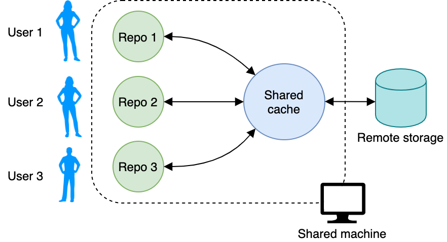
Great. Now you have a shared cache that all other users can share for their repositories. If your operating system (OS) doesn’t allow everyone to work with the shared cache, then make sure all the permissions on your system are set correctly. You can find more details on setting up a shared system in the DVC docs.
If you check your repository’s .dvc/config file, then you’ll see a new section appear:
[cache]
    dir = /path/to/shared_cache
This allows you to double-check where your data gets backed up.
But how does this help you save space? Instead of having copies of the same data in your local repository, the shared cache, and all the other repositories on the machine, DVC can use links. Links are a feature of operating systems.
If you have a file, like an image, then you can create a link to that file. The link looks just like another file on your system, but it doesn’t contain the data. It only refers to the actual file somewhere else on the system, like a shortcut. There are many types of links, like reflinks, symlinks, and hardlinks. Each has different properties.
DVC will try to use reflinks by default, but they’re not available on all computers. If your OS doesn’t support reflinks, DVC will default to creating copies. You can learn more about file link types in the DVC docs.
You can change the default behavior of your cache by changing the cache.type configuration option:
$ dvc config cache.type symlink
You can replace symlink with reflink, hardlink, or copies. Research each type of link and choose the most appropriate option for the OS you’re working on. Remember, you can check how your DVC repository is currently configured by reading the .dvc/config file:
[cache]
    dir = /path/to/shared_cache
    type = symlink
If you make a change to the cache.type, it doesn’t take effect immediately. You need to tell DVC to check out links instead of file copies:
$ dvc checkout --relink
The --relink switch will tell DVC to check the cache type and relink all the files that are currently tracked by DVC.
If there are models or data files in your repository or cache that aren’t being used, then you can save additional space by cleaning up your repository with dvc gc. gc stands for garbage collection and will remove any unused files and directories from the cache.
Important: Be careful with any commands that delete data!
Make sure you understand all the nuances by consulting the official docs for commands that remove files, such as gc and remove.
You’re now all set to share a development machine with your team. The next feature to explore is creating pipelines.
Create Reproducible Pipelines
Here’s a recap of the steps you made so far to train your machine learning model:
- Fetching the data
- Preparing the data
- Running training
- Evaluating the training run
You fetched the data manually and added it to remote storage. You can now get it with dvc checkout or dvc pull. The other steps were executed by running various Python files. These can be chained together into a single execution called a DVC pipeline that requires only one command.
Create a new branch and call it sgd-pipeline:
$ git checkout -b sgd-pipeline
You’ll use this branch to rerun the experiment as a DVC pipeline. A pipeline consists of multiple stages and is executed using a dvc run command. Each stage has three components:
- Inputs
- Outputs
- Command
DVC uses the term dependencies for inputs and outs for outputs. The command can be anything you usually run in the command line, including Python files. You can practice creating a pipeline of stages while running another experiment. Each of your three Python files, prepare.py, train.py, and evaluate.py will be represented by a stage in the pipeline.
Note: You’re going to reproduce all the files you created with prepare.py, train.py, and evaluate.py by creating pipelines.
A pipeline automatically adds newly created files to DVC control, just as if you’ve typed dvc add. Since you’ve manually added a lot of your files to DVC control already, DVC will get confused if you try to create the same files using a pipeline.
To avoid that, first remove the CSV files, models, and metrics using dvc remove:
$ dvc remove data/prepared/train.csv.dvc \
             data/prepared/test.csv.dvc \
             model/model.joblib.dvc --outs
This will remove the .dvc files and the associated data targeted by the .dvc files. You should now have a blank slate to re-create these files using DVC pipelines.
First, you’re going to run prepare.py as a DVC pipeline stage. The command for this is dvc run, which needs to know the dependencies, outputs, and command:
- Dependencies:
prepare.pyand the data indata/raw - Outputs:
train.csvandtest.csv - Command:
python prepare.py
Execute prepare.py as a DVC pipeline stage with the dvc run command:
 1$ dvc run -n prepare \
 2        -d src/prepare.py -d data/raw \
 3        -o data/prepared/train.csv -o data/prepared/test.csv \
 4        python src/prepare.py
All this is a single command. The first row starts the dvc run command and accepts a few options:
- The
-nswitch gives the stage a name. - The
-dswitch passes the dependencies to the command. - The
-oswitch defines the outputs of the command.
The main argument to the command is the Python command that will be executed, python src/prepare.py. In plain English, the above dvc run command gives DVC the following information:
- Line 1: You want to run a pipeline stage and call it
prepare. - Line 2: The pipeline needs the
prepare.pyfile and thedata/rawfolder. - Line 3: The pipeline will produce the
train.csvandtest.csvfiles. - Line 4: The command to execute is
python src/prepare.py.
Once you create the stage, DVC will create two files, dvc.yaml and dvc.lock. Open them and take a look inside.
This is an example of what you’ll see in dvc.yaml:
stages:
  prepare:
    cmd: python src/prepare.py
    deps:
      - data/raw
      - src/prepare.py
    outs:
      - data/prepared/test.csv
      - data/prepared/train.csv
It’s all the information you put in the dvc run command. The top-level element, stages, has elements nested under it, one for each stage. Currently, you have only one stage, prepare. As you chain more, they’ll show up in this file. Technically, you don’t have to type dvc run commands in the command line—you can create all your stages here.
Every dvc.yaml has a corresponding dvc.lock file, which is also in the YAML format. The information inside is similar, with the addition of MD5 hashes for all dependencies and outputs:
prepare:
  cmd: python src/prepare.py
  deps:
    - path: data/raw
      md5: a8a5252d9b14ab2c1be283822a86981a.dir
    - path: src/prepare.py
      md5: 0e29f075d51efc6d280851d66f8943fe
  outs:
    - path: data/prepared/test.csv
      md5: d4a8cdf527c2c58d8cc4464c48f2b5c5
    - path: data/prepared/train.csv
      md5: 50cbdb38dbf0121a6314c4ad9ff786fe
Adding MD5 hashes allows DVC to track all dependencies and outputs and detect if any of these files change. For example, if a dependency file changes, then it will have a different hash value, and DVC will know it needs to rerun that stage with the new dependency. So instead of having individual .dvc files for train.csv, test.csv, and model.joblib, everything is tracked in the .lock file.
Great—you’ve automated the first stage of the pipeline, which can be visualized as a flow diagram:
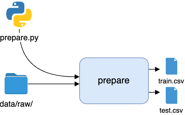
You’ll use the CSV files produced by this stage in the following stage.
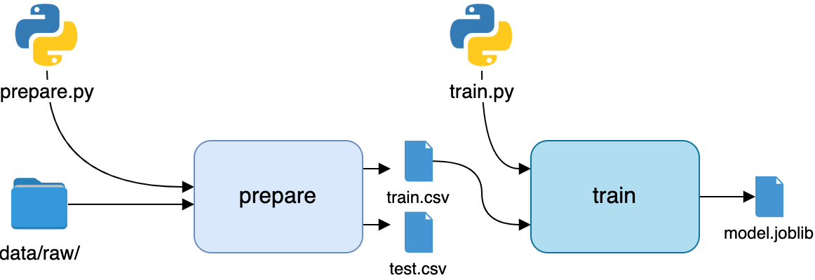
The next stage in the pipeline is training. The dependencies are the train.py file itself and the train.csv file in data/prepared. The only output is the model.joblib file. To create a pipeline stage out of train.py, execute it with dvc run, specifying the correct dependencies and outputs:
$ dvc run -n train \
        -d src/train.py -d data/prepared/train.csv \
        -o model/model.joblib \
        python src/train.py
This will create the second stage of the pipeline and record it in the dvc.yml and dvc.lock files. Here’s a visualization of the new state of the pipeline:
Two down, one to go! The final stage will be the evaluation. The dependencies are the evaluate.py file and the model file generated in the previous stage. The output is the metrics file, accuracy.json. Execute evaluate.py with dvc run:
$ dvc run -n evaluate \
        -d src/evaluate.py -d model/model.joblib \
        -M metrics/accuracy.json \
        python src/evaluate.py
Notice that you used the -M switch instead of -o. DVC treats metrics differently from other outputs. When you run this command, it will generate the accuracy.json file, but DVC will know that it’s a metric used to measure the performance of the model.
You can get DVC to show you all the metrics it knows about with the dvc show command:
$ dvc metrics show
        metrics/accuracy.json:
            accuracy: 0.6996197718631179
You’ve completed the final stage of the pipeline, which looks like this:
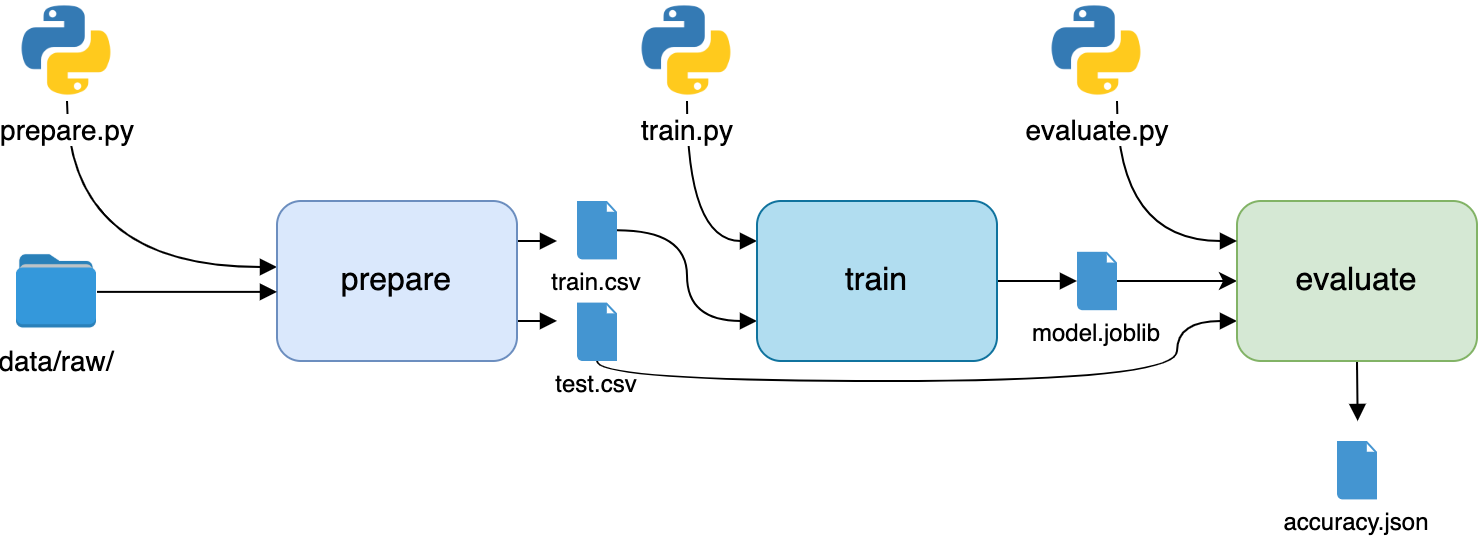
You can now see your entire workflow in a single image. Don’t forget to tag your new branch and push all the changes to GitHub and DVC:
$ git add --all
$ git commit -m "Rerun SGD as pipeline"
$ dvc commit
$ git push --set-upstream origin sgd-pipeline
$ git tag -a sgd-pipeline -m "Trained SGD as DVC pipeline."
$ git push origin --tags
$ dvc push
This will version and store your code, models, and data for the new DVC pipeline.
Now for the best part!
For training, you’ll use a random forest classifier, which is a different model that can be used for classification. It’s more complex than the SGDClassifier and could potentially yield better results. Start by creating and checking out a new branch and calling it random_forest:
$ git checkout -b "random_forest"
The power of pipelines is the ability to reproduce them with minimal hassle whenever you change anything. Modify your train.py to use a RandomForestClassifier instead of the SGDClassifier:
# train.py
from joblib import dump
from pathlib import Path

import numpy as np
import pandas as pd
from skimage.io import imread_collection
from skimage.transform import resize
from sklearn.ensemble import RandomForestClassifier
# ...

def main(path_to_repo):
    train_csv_path = repo_path / "data/prepared/train.csv"
    train_data, labels = load_data(train_csv_path)
    rf = RandomForestClassifier()
    trained_model = rf.fit(train_data, labels)
    dump(trained_model, repo_path / "model/model.joblib")
The only lines that changed were importing the RandomForestClassifier instead of the SGDClassifier, creating an instance of the classifier, and calling its fit() method. Everything else remained the same.
Since your train.py file changed, its MD5 hash has changed. DVC will realize that one of the pipeline stages needs to be reproduced. You can check what changed with the dvc status command:
$ dvc status
train:
    changed deps:
        modified:           src/train.py
This will display all the changed dependencies for every stage of the pipeline. Since the change in the model will affect the metric as well, you want to reproduce the whole chain. You can reproduce any DVC pipeline file with the dvc repro command:
$ dvc repro evaluate
And that’s it! When you run the repro command, DVC checks all the dependencies of the entire pipeline to determine what’s changed and which commands need to be executed again. Think about what this means. You can jump from branch to branch and reproduce any experiment with a single command!
To wrap up, push your random forest classifier code to GitHub and the model to DVC:
$ git add --all
$ git commit -m "Train Random Forrest classifier"
$ dvc commit
$ git push --set-upstream origin random-forest
$ git tag -a random-forest -m "Random Forest classifier with 80.99% accuracy."
$ git push origin --tags
$ dvc push
Now you can compare metrics across multiple branches and tags.
Call dvc metrics show with the -T switch to display metrics across multiple tags:
$ dvc metrics show -T
sgd-pipeline:
    metrics/accuracy.json:
        accuracy: 0.6996197718631179
forest:
    metrics/accuracy.json:
        accuracy: 0.8098859315589354
Awesome! This gives you a quick way to keep track of what the best-performing experiment was in your repository.
When you come back to this project in six months and don’t remember the details, you can check which setup was the most successful with dvc metrics show -T and reproduce it with dvc repro! Anyone else who wants to reproduce your work can do the same. They’ll just need to take three steps:
- Run
git cloneorgit checkoutto get the code and.dvcfiles. - Get the training data with
dvc checkout. - Reproduce the entire workflow with
dvc repro evaluate.
If they can write a script to fetch the data and create a pipeline stage for it, then they won’t even need step 2.
Nice work! You ran multiple experiments and safely versioned and backed up the data and models. What’s more, you can quickly reproduce each experiment by just getting the necessary code and data and executing a single dvc repro command.
Next Steps
Congratulations on completing the tutorial! You’ve learned how to use data version control in your daily work. If you want to go deeper into optimizing your workflow or learning more about DVC, then this section offers some suggestions.
Remembering to run all the DVC and Git commands at the right time can be a challenge, especially when you’re just getting started. DVC offers the possibility to integrate the two tighter together. Using Git hooks, you can execute DVC commands automatically when you run certain Git commands. Read more about installing Git hooks for DVC in the official docs.
Git and GitHub allow you to track the history of changes for a particular repository. You can see who updated what and when. You can create pull requests to update data. Patterns like these are possible with DVC as well. Have a look at the section on data registries in the DVC docs.
DVC even has a Python API, which means you can call DVC commands in your Python code to access data or models stored in DVC repositories.
Even though this tutorial provides a broad overview of the possibilities of DVC, it’s impossible to cover everything in a single document. You can explore DVC in detail by checking out the official User Guide, Command Reference, and Interactive Tutorials.
Conclusion
You now know how to use DVC to solve problems data scientists have been struggling with for years! For every experiment you run, you can version the data you use and the model you train. You can share training machines with other team members without fear of losing your data or running out of disk space. Your experiments are reproducible, and anyone can repeat what you’ve done.
In this tutorial, you’ve learned how to:
- Use DVC in a workflow similar to Git, with
add,commit, andpushcommands - Share development machines with other team members and save space with symlinks
- Create experiment pipelines that can be reproduced with
dvc repro
If you’d like to reproduce the examples you saw above, then be sure to download the source code by clicking the following link:
Get the Source Code: Click here to get the source code you’ll use to learn about data version control with DVC in this tutorial.
Practice these techniques and you’ll start doing this process automatically. This will allow you to put all your focus into running cool experiments. Good luck!


