Tutorial
How To Trick a Neural Network in Python 3

The author selected Dev Color to receive a donation as part of the Write for DOnations program.
Could a neural network for animal classification be fooled? Fooling an animal classifier may have few consequences, but what if our face authenticator could be fooled? Or our self-driving car prototype’s software? Fortunately, legions of engineers and research stand between a prototype computer-vision model and production-quality models on our mobile devices or cars. Still, these risks have significant implications and are important to consider as a machine-learning practitioner.
In this tutorial, you will try “fooling” or tricking an animal classifier. As you work through the tutorial, you’ll use OpenCV, a computer-vision library, and PyTorch, a deep learning library. You will cover the following topics in the associated field of adversarial machine learning:
- Create a targeted adversarial example. Pick an image, say, of a dog. Pick a target class, say, a cat. Your goal is to trick the neural network into believing the pictured dog is a cat.
- Create an adversarial defense. In short, protect your neural network against these tricky images, without knowing what the trick is.
By the end of the tutorial, you will have a tool for tricking neural networks and an understanding of how to defend against tricks.
Prerequisites
To complete this tutorial, you will need the following:
- A local development environment for Python 3 with at least 1GB of RAM. You can follow How to Install and Set Up a Local Programming Environment for Python 3 to configure everything you need.
- It is recommended that you review Build an Emotion-Based Dog Filter; this tutorial is not explicitly used but introduces the notion of classification.
Step 1 — Creating Your Project and Installing Dependencies
Let’s create a workspace for this project and install the dependencies you’ll need. You’ll call your workspace AdversarialML:
- mkdir ~/AdversarialML
Navigate to the AdversarialML directory:
- cd ~/AdversarialML
Make a directory to hold all your assets:
- mkdir ~/AdversarialML/assets
Then create a new virtual environment for the project:
- python3 -m venv adversarialml
Activate your environment:
- source adversarialml/bin/activate
Then install PyTorch, a deep-learning framework for Python that you’ll use in this tutorial.
On macOS, install Pytorch with the following command:
- python -m pip install torch==1.2.0 torchvision==0.4.0
On Linux and Windows, use the following commands for a CPU-only build:
- pip install torch==1.2.0+cpu torchvision==0.4.0+cpu -f https://download.pytorch.org/whl/torch_stable.html
- pip install torchvision
Now install prepackaged binaries for OpenCV and numpy, which are libraries for computer vision and linear algebra, respectively. OpenCV offers utilities such as image rotations, and numpy offers linear algebra utilities such as a matrix inversion:
- python -m pip install opencv-python==3.4.3.18 numpy==1.14.5
On Linux distributions, you will need to install libSM.so:
- sudo apt-get install libsm6 libxext6 libxrender-dev
With the dependencies installed, let’s run an animal classifier called ResNet18, which we describe next.
Step 2 — Running a Pretrained Animal Classifier
The torchvision library, the official computer vision library for PyTorch, contains pretrained versions of commonly used computer vision neural networks. These neural networks are all trained on ImageNet 2012, a dataset of 1.2 million training images with 1000 classes. These classes include vehicles, places, and most importantly, animals. In this step, you will run one of these pretrained neural networks, called ResNet18. We will refer to ResNet18 trained on ImageNet as an “animal classifier”.
What is ResNet18? ResNet18 is the smallest neural network in a family of neural networks called residual neural networks, developed by MSR (He et al.). In short, He found that a neural network (denoted as a function f, with input x, and output f(x)) would perform better with a “residual connection” x + f(x). This residual connection is used prolifically in state-of-the-art neural networks, even today. For example, FBNetV2, FBNetV3.
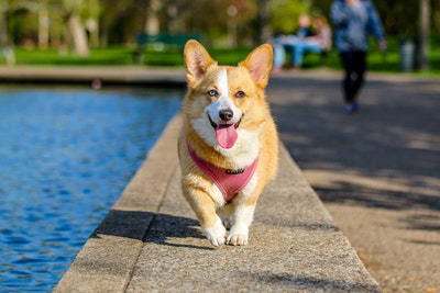
Download this image of a dog with the following command:
- wget -O assets/dog.jpg https://assets.digitalocean.com/articles/trick_neural_network/step2a.png
Then, download a JSON file to convert neural network output to a human-readable class name:
- wget -O assets/imagenet_idx_to_label.json https://raw.githubusercontent.com/do-community/tricking-neural-networks/master/utils/imagenet_idx_to_label.json
Next, create a script to run your pretrained model on the dog image. Create a new file called step_2_pretrained.py:
- nano step_2_pretrained.py
First, add the Python boilerplate by importing the necessary packages and declaring a main function:
from PIL import Image
import json
import torchvision.models as models
import torchvision.transforms as transforms
import torch
import sys

def main():
    pass

if __name__ == '__main__':
    main()
Next, load the mapping from neural network output to human-readable class names. Add this directly after your import statements and before your main function:
. . .
def get_idx_to_label():
    with open("assets/imagenet_idx_to_label.json") as f:
        return json.load(f)
. . .
Create an image transformation function that will ensure your input image firstly has the correct dimensions, and secondly is normalized correctly. Add the following function directly after the last:
. . .
def get_image_transform():
    transform = transforms.Compose([
      transforms.Resize(224),
      transforms.CenterCrop(224),
      transforms.ToTensor(),
      transforms.Normalize(mean=[0.485, 0.456, 0.406],
                           std=[0.229, 0.224, 0.225])
    ])
    return transform
. . .
In get_image_transform, you define a number of different transformations to apply to the images that are passed to your neural network:
transforms.Resize(224): Resizes the smaller side of the image to 224. For example, if your image is 448 x 672, this operation would downsample the image to 224 x 336.transforms.CenterCrop(224): Takes a crop from the center of the image, of size 224 x 224.transforms.ToTensor(): Converts the image into a PyTorch tensor. All PyTorch models require PyTorch tensors as input.transforms.Normalize(mean=..., std=...): Standardizes your input by subtracting the mean, then dividing by the standard deviation. This is described more precisely in thetorchvisiondocumentation.
Add a utility to predict the animal class, given the image. This method uses both the previous utilities to perform animal classification:
. . .
def predict(image):
    model = models.resnet18(pretrained=True)
    model.eval()

    out = model(image)

    _, pred = torch.max(out, 1)
    idx_to_label = get_idx_to_label()
    cls = idx_to_label[str(int(pred))]
    return cls
. . .
Here the predict function classifies the provided image using a pretrained neural network:
models.resnet18(pretrained=True): Loads a pretrained neural network called ResNet18.model.eval(): Modifies the model in-place to run in ‘evaluation’ mode. The only other mode is ‘training’ mode, but training mode isn’t needed, as you aren’t training the model (that is, updating the model’s parameters) in this tutorial.out = model(image): Runs the neural network on the provided, transformed image._, pred = torch.max(out, 1): The neural network outputs one probability for each possible class. This step computes the index of the class with the highest probability. For example, ifout = [0.4, 0.1, 0.2], thenpred = 0.idx_to_label = get_idx_to_label(): Obtains a mapping from class index to human-readable class names. For example, the mapping could be{0: cat, 1: dog, 2: fish}.cls = idx_to_label[str(int(pred))]: Convert the predicted class index to a class name. The examples provided in the last two bullet points would yieldcls = idx_to_label[0] = 'cat'.
Next, following the last function, add a utility to load images:
. . .
def load_image():
    assert len(sys.argv) > 1, 'Need to pass path to image'
    image = Image.open(sys.argv[1])

    transform = get_image_transform()
    image = transform(image)[None]
    return image
. . .
This will load an image from the path provided in the first argument to the script. transform(image)[None] applies the sequence of image transformations defined in the previous lines.
Finally, populate your main function with the following, to load your image and classify the animal in the image:
def main():
    x = load_image()
    print(f'Prediction: {predict(x)}')
Double check that your file matches our final step 2 script at step_2_pretrained.py on GitHub. Save and exit your script, and run the animal classifier:
- python step_2_pretrained.py assets/dog.jpg
This will produce the following output, showing your animal classifier works as expected:
OutputPrediction: Pembroke, Pembroke Welsh corgi
That concludes running inference with your pretrained model. Next, you will see an adversarial example in action by tricking a neural network with impercetible differences in the image.
Step 3 — Trying an Adversarial Example
Now, you will synthesize an adversarial example, and test the neural network on that example. For this tutorial, you will build adversarial examples of the form x + r, where x is the original image and r is some “perturbation”. You will eventually create the perturbation r yourself, but in this step, you will download one we created for you beforehand. Start by downloading the perturbation r:
- wget -O assets/adversarial_r.npy https://github.com/do-community/tricking-neural-networks/blob/master/outputs/adversarial_r.npy?raw=true
Now composite the picture with the perturbation. Create a new file called step_3_adversarial.py:
- nano step_3_adversarial.py
In this file, you will perform the following three-step process, to produce an adversarial example:
- Transform an image
- Apply the perturbation
r - Inverse transform the perturbed image
At the end of step 3, you will have an adversarial image. First, import the necessary packages and declare a main function:
from PIL import Image
import torchvision.transforms as transforms
import torch
import numpy as np
import os
import sys

from step_2_pretrained import get_idx_to_label, get_image_transform, predict, load_image


def main():
    pass


if __name__ == '__main__':
    main()
Next, create an “image transformation” that inverts the earlier image transformation. Place this after your imports, before the main function:
. . .
def get_inverse_transform():
    return transforms.Normalize(
        mean=[-0.485/0.229, -0.456/0.224, -0.406/0.255],  # INVERSE normalize images, according to https://pytorch.org/docs/stable/torchvision/models.html
        std=[1/0.229, 1/0.224, 1/0.255])
. . .
As before, the transforms.Normalize operation subtracts the mean and divides by the standard deviation (that is, for the original image x, y = transforms.Normalize(mean=u, std=o) = (x - u) / o). You do some algebra and define a new operation that reverses this normalize function (transforms.Normalize(mean=-u/o, std=1/o) = (y - -u/o) / 1/o = (y + u/o) o = yo + u = x).
As part of the inverse transformation, add a method that transforms a PyTorch tensor back to a PIL image. Add this following the last function:
. . .
def tensor_to_image(tensor):
    x = tensor.data.numpy().transpose(1, 2, 0) * 255.
    x = np.clip(x, 0, 255)
    return Image.fromarray(x.astype(np.uint8))
. . .
tensor.data.numpy()converts the PyTorch tensor into a NumPy array..transpose(1, 2, 0)rearranges(channels, width, height)into(height, width, channels). This NumPy array is approximately in the range(0, 1). Finally, multiply by 255 to ensure the image is now in the range(0, 255).np.clipensures that all values in the image are between(0, 255).x.astype(np.uint8)ensures all image values are integers. Finally,Image.fromarray(...)creates a PIL image object from the NumPy array.
Then, use these utilities to create the adversarial example with the following:
. . .
def get_adversarial_example(x, r):
    y = x + r
    y = get_inverse_transform()(y[0])
    image = tensor_to_image(y)
    return image
. . .
This function generates the adversarial example as described at the start of the section:
y = x + r. Take your perturbationrand add it to the original imagex.get_inverse_transform: Obtain and apply the reverse image transformation you defined several lines earlier.tensor_to_image: Finally, convert the PyTorch tensor back to an image object.
Finally, modify your main function to load the image, load the adversarial perturbation r, apply the perturbation, save the adversarial example to disk, and run prediction on the adversarial example:
def main():
    x = load_image()
    r = torch.Tensor(np.load('assets/adversarial_r.npy'))

    # save perturbed image
    os.makedirs('outputs', exist_ok=True)
    adversarial = get_adversarial_example(x, r)
    adversarial.save('outputs/adversarial.png')

    # check prediction is new class
    print(f'Old prediction: {predict(x)}')
    print(f'New prediction: {predict(x + r)}')
Your completed file should match step_3_adversarial.py on GitHub. Save the file, exit the editor, and launch your script with:
- python step_3_adversarial.py assets/dog.jpg
You’ll see this output:
OutputOld prediction: Pembroke, Pembroke Welsh corgi
New prediction: goldfish, Carassius auratus
You’ve now created an adversarial example: tricking the neural network into thinking a corgi is a goldfish. In the next step, you will actually create the perturbation r that you used here.
Step 4 — Understanding an Adversarial Example
For a primer on classification, see “How to Build an Emotion-Based Dog Filter”.
Taking a step back, recall that your classification model outputs a probability for each class. During inference, the model predicts the class with the highest probability. During training, you update the model parameters t to maximize the probability of the correct class y, given your data x.
argmax_y P(y|x,t)
However, to generate adversarial examples, you now modify your goal. Instead of finding a class, your goal is now to find a new image, x. Take any class other than the correct one. Let us call this new class w. Your new objective is to maximize the probability of the wrong class.
argmax_x P(w|x)
Note that the neural network weights t are missing from the above expression. This is because you now assume the role of the adversary: Someone else has trained and deployed a model. You are only allowed to create adversarial inputs and are not allowed to modify the deployed model. To generate the adversarial example x, you can run “training”, except instead of updating the neural network weights, you update the input image with the new objective.
As a reminder, for this tutorial, you assume that the adversarial example is an affine transformation of x. In other words, your adversarial example takes the form x + r for some r. In the next step, you will write a script to generate this r.
Step 5 — Creating an Adversarial Example
In this step, you will learn a perturbation r, so that your corgi is misclassified as a goldfish. Create a new file called step_5_perturb.py:
- nano step_5_perturb.py
Import the necessary packages and declare a main function:
from torch.autograd import Variable
import torchvision.models as models
import torch.nn as nn
import torch.optim as optim
import numpy as np
import torch
import os

from step_2_pretrained import get_idx_to_label, get_image_transform, predict, load_image
from step_3_adversarial import get_adversarial_example


def main():
    pass


if __name__ == '__main__':
    main()
Directly following your imports and before the main function, define two constants:
. . .
TARGET_LABEL = 1
EPSILON = 10 / 255.
. . .
The first constant TARGET_LABEL is the class to misclassify the corgi as. In this case, index 1 corresponds to “goldfish”. The second constant EPSILON is the maximum amount of perturbation allowed for each image value. This limit is introduced so that the image is imperceptibly altered.
Following your two constants, add a helper function to define a neural network and the perturbation parameter r:
. . .
def get_model():
    net = models.resnet18(pretrained=True).eval()
    r = nn.Parameter(data=torch.zeros(1, 3, 224, 224), requires_grad=True)
    return net, r
. . .
model.resnet18(pretrained=True)loads a pretrained neural network called ResNet18, like before. Also like before, you set the model to evaluation mode using.eval.nn.Parameter(...)defines a new perturbationr, the size of the input image. The input image is also of size(1, 3, 224, 224). Therequires_grad=Truekeyword argument ensures that you can update this perturbationrin later lines, in this file.
Next, begin modifying your main function. Start by loading the model net, loading the inputs x, and defining the label label:
. . .
def main():
    print(f'Target class: {get_idx_to_label()[str(TARGET_LABEL)]}')
    net, r = get_model()
    x = load_image()
    labels = Variable(torch.Tensor([TARGET_LABEL])).long()
  . . .
Next, define both the criterion and the optimizer in your main function. The former tells PyTorch what the objective is—that is, what loss to minimize. The latter tells PyTorch how to train your parameter r:
. . .
    criterion = nn.CrossEntropyLoss()
    optimizer = optim.SGD([r], lr=0.1, momentum=0.1)
. . .
Directly following, add the main training loop for your parameter r:
. . .
    for i in range(30):
        r.data.clamp_(-EPSILON, EPSILON)
        optimizer.zero_grad()

        outputs = net(x + r)
        loss = criterion(outputs, labels)
        loss.backward()
        optimizer.step()

        _, pred = torch.max(outputs, 1)
        if i % 5 == 0:
            print(f'Loss: {loss.item():.2f} / Class: {get_idx_to_label()[str(int(pred))]}')
. . .
On each iteration of this training loop, you:
r.data.clamp_(...): Ensure the parameterris small, withinEPSILONof 0.optimizer.zero_grad(): Clear any gradients you computed in the previous iteration.model(x + r): Run inference on the modified imagex + r.- Compute the
loss. - Compute the gradient
loss.backward. - Take a gradient descent step
optimizer.step. - Compute the prediction
pred. - Finally, report the loss and predicted class
print(...).
Next, save the final perturbation r:
def main():
    . . .
    for i in range(30):
        . . .
    . . .
    np.save('outputs/adversarial_r.npy', r.data.numpy())
Directly following, still in the main function, save the perturbed image:
. . .
    os.makedirs('outputs', exist_ok=True)
    adversarial = get_adversarial_example(x, r)
Finally, run prediction on both the original image and the adversarial example:
    print(f'Old prediction: {predict(x)}')
    print(f'New prediction: {predict(x + r)}')
Double check your script matches step_5_perturb.py on GitHub. Save, exit, and run the script:
- python step_5_perturb.py assets/dog.jpg
Your script will output the following.
OutputTarget class: goldfish, Carassius auratus
Loss: 17.03 / Class: Pembroke, Pembroke Welsh corgi
Loss: 8.19 / Class: Pembroke, Pembroke Welsh corgi
Loss: 5.56 / Class: Pembroke, Pembroke Welsh corgi
Loss: 3.53 / Class: Pembroke, Pembroke Welsh corgi
Loss: 1.99 / Class: Pembroke, Pembroke Welsh corgi
Loss: 1.00 / Class: goldfish, Carassius auratus
Old prediction: Pembroke, Pembroke Welsh corgi
New prediction: goldfish, Carassius auratus
The last two lines indicate you have now completed construction of an adversarial example from scratch. Your neural network now classifies a perfectly reasonable corgi image as a goldfish.
You’ve now shown that neural networks can be fooled easily—what’s more, the lack of robustness to adversarial examples has significant consequences. A natural next question is this: How can you combat adversarial examples? A good amount of research has been conducted by various organizations, including OpenAI. In the next section, you’ll run a defense to thwart this adversarial example.
Step 6 — Defending Against Adversarial Examples
In this step, you will implement a defense against adversarial examples. The idea is the following: You are now the owner of the animal classifier being deployed to production. You don’t know what adversarial examples may be generated, but you can modify the image or the model to protect against attacks.
Before you defend, you should see for yourself how imperceptible the image manipulation is. Open both of the following images:
assets/dog.jpgoutputs/adversarial.png
Here, you show both side by side. Your original image will have a different aspect ratio. Can you tell which is the adversarial example?
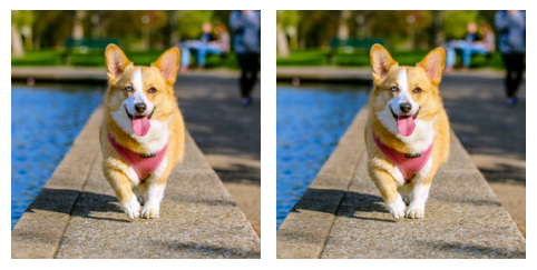
Notice that the new image looks identical to the original. As it turns out, the left image is your adversarial image. To be certain, download the image and run your evaluation script:
- wget -O assets/adversarial.png https://github.com/alvinwan/fooling-neural-network/blob/master/outputs/adversarial.png?raw=true
- python step_2_pretrained.py assets/adversarial.png
This will output the goldfish class, to prove its adversarial nature:
OutputPrediction: goldfish, Carassius auratus
You will run a fairly naive, but effective, defense: Compress the image by writing to a lossy JPEG format. Open the Python interactive prompt:
- python
Then, load the adversarial image as PNG, and save it back as a JPEG.
- from PIL import Image
- image = Image.open('assets/adversarial.png')
- image.save('outputs/adversarial.jpg')
Type CTRL + D to leave the Python interactive prompt. Next, run inference with your model on the compressed adversarial example:
- python step_2_pretrained.py outputs/adversarial.jpg
This will now output the corgi class, proving the efficacy of your naive defense.
OutputPrediction: Pembroke, Pembroke Welsh corgi
You’ve now completed your very first adversarial defense. Note that this defense does not require knowing how the adversarial example was generated. This is what makes an effective defense. There are also many other forms of defense, many of which involve retraining the neural network. However, these retraining procedures are a topic of their own and beyond the scope of this tutorial. With that, this concludes your guide into adversarial machine learning.
Conclusion
To understand the implications of your work in this tutorial, revisit the two images side-by-side—the original and the adversarial example.
Despite the fact that both images look identical to the human eye, the first has been manipulated to fool your model. Both images clearly feature a corgi, and yet the model is entirely confident that the second model contains a goldfish. This should concern you and, as you wrap up this tutorial, keep in mind the fragility of your model. Just by applying a simple transformation, you can fool it. These are real, plausible dangers that evade even cutting-edge research. Research beyond machine-learning security is just as susceptible to these flaws, and, as a practitioner, it is up to you to apply machine learning safely. For more readings, check out the following links:
- Adversarial Machine Learning tutorial from NeurIPS 2018 Conference.
- Related blog posts from OpenAI on Attacking Machine Learning with Adversarial Examples, Testing Robustness Against Unseen Adversaries, and Robust Adversarial Inputs.
For more machine learning content and tutorials, you can visit our Machine Learning Topic page.
Thanks for learning with the DigitalOcean Community. Check out our offerings for compute, storage, networking, and managed databases.
author
AI PhD Student @ UC Berkeley
I’m a diglot by definition, lactose intolerant by birth but an ice-cream lover at heart. Call me wabbly, witling, whatever you will, but I go by Alvin
editor
This textbox defaults to using Markdown to format your answer.
You can type !ref in this text area to quickly search our full set of tutorials, documentation & marketplace offerings and insert the link!


Get our biweekly newsletter
Sign up for Infrastructure as a Newsletter.

Hollie's Hub for Good
Working on improving health and education, reducing inequality, and spurring economic growth? We'd like to help.

Become a contributor
Get paid to write technical tutorials and select a tech-focused charity to receive a matching donation.
