Scientific Python: Using SciPy for Optimization

When you want to do scientific work in Python, the first library you can turn to is SciPy. As you’ll see in this tutorial, SciPy is not just a library, but a whole ecosystem of libraries that work together to help you accomplish complicated scientific tasks quickly and reliably.

In this tutorial, you’ll learn how to:

Find information about all the things you can do with SciPy
Install SciPy on your computer
Use SciPy to cluster a dataset by several variables
Use SciPy to find the optimum of a function

You can follow along with the examples in this tutorial by downloading the source code available at the link below:

Get Sample Code: Click here to get the sample code you’ll use to learn about SciPy in this tutorial.

Differentiating SciPy the Ecosystem and SciPy the Library

When you want to use Python for scientific computing tasks, there are several libraries that you’ll probably be advised to use, including:

NumPy
SciPy
Matplotlib
IPython
SymPy
Pandas

Collectively, these libraries make up the SciPy ecosystem and are designed to work together. Many of them rely directly on NumPy arrays to do computations. This tutorial expects that you have some familiarity with creating NumPy arrays and operating on them.

Note: If you need a quick primer or refresher on NumPy, then you can check out these tutorials:

In this tutorial, you’ll learn about the SciPy library, one of the core components of the SciPy ecosystem. The SciPy library is the fundamental library for scientific computing in Python. It provides many efficient and user-friendly interfaces for tasks such as numerical integration, optimization, signal processing, linear algebra, and more.

Remove ads

Understanding SciPy Modules

The SciPy library is composed of a number of modules that separate the library into distinct functional units. If you want to learn about the different modules that SciPy includes, then you can run help() on scipy, as shown below:

Python
      
>>> import scipy
>>> help(scipy)

This produces some help output for the entire SciPy library, a portion of which is shown below:

Text

Subpackages
-----------

Using any of these subpackages requires an explicit import.  For example,
``import scipy.cluster``.

::

 cluster                      --- Vector Quantization / Kmeans
 fft                          --- Discrete Fourier transforms
 fftpack                      --- Legacy discrete Fourier transforms
 integrate                    --- Integration routines
...

This code block shows the Subpackages portion of the help output, which is a list of all of the available modules within SciPy that you can use for calculations.

Note the text at the top of the section that states, "Using any of these subpackages requires an explicit import." When you want to use functionality from a module in SciPy, you need to import the module that you want to use specifically. You’ll see some examples of this a little later in the tutorial, and guidelines for importing libraries from SciPy are shown in the SciPy documentation.

Once you decide which module you want to use, you can check out the SciPy API reference, which contains all of the details on each module in SciPy. If you’re looking for something with a little more exposition, then the SciPy Lecture Notes are a great resource to go in-depth on many of the SciPy modules.

Later in this tutorial, you’ll learn about cluster and optimize, which are two of the modules in the SciPy library. But first, you’ll need to install SciPy on your computer.

Installing SciPy on Your Computer

As with most Python packages, there are two main ways to install SciPy on your computer:

Here, you’ll learn how to use both of these approaches to install the library. SciPy’s only direct dependency is the NumPy package. Either installation method will automatically install NumPy in addition to SciPy, if necessary.

Anaconda

Anaconda is a popular distribution of Python, mainly because it includes pre-built versions of the most popular scientific Python packages for Windows, macOS, and Linux. If you don’t have Python installed on your computer at all yet, then Anaconda is a great option to get started with. Anaconda comes pre-installed with SciPy and its required dependencies, so once you’ve installed Anaconda, you don’t need to do anything else!

You can download and install Anaconda from their downloads page. Make sure to download the most recent Python 3 release. Once you have the installer on your computer, you can follow the default setup procedure for an application, depending on your platform.

Note: Make sure to install Anaconda in a directory that does not require administrator permissions to modify. This is the default setting in the installer.

If you already have Anaconda installed, but you want to install or update SciPy, then you can do that, too. Open up a terminal application on macOS or Linux, or the Anaconda Prompt on Windows, and type one of the following lines of code:

Shell
      
$ conda install scipy
$ conda update scipy

You should use the first line if you need to install SciPy or the second line if you just want to update SciPy. To make sure SciPy is installed, run Python in your terminal and try to import SciPy:

Python
      
>>> import scipy
>>> print(scipy.__file__)
/.../lib/python3.7/site-packages/scipy/__init__.py

In this code, you’ve imported scipy and printed the location of the file from where scipy is loaded. The example above is for macOS. Your computer will probably show a different location. Now you have SciPy installed on your computer ready for use. You can skip ahead to the next section to get started using SciPy!

Remove ads

The `pip` Package Manager

If you already have a version of Python installed that isn’t Anaconda, or you don’t want to use Anaconda, then you’ll be using pip to install SciPy. To learn more about what pip is, check out Using Python’s pip to Manage Your Projects’ Dependencies and A Beginner’s Guide to pip.

Note: pip installs packages using a format called wheels. In the wheel format, code is compiled before it’s sent to your computer. This is nearly the same approach that Anaconda takes, although wheel format files are slightly different than the Anaconda format, and the two are not interchangeable.

To install SciPy using pip, open up your terminal application, and type the following line of code:

Shell
      
$ python -m pip install -U scipy

The code will install SciPy if it isn’t already installed, or upgrade SciPy if it is installed. To make sure SciPy is installed, run Python in your terminal and try to import SciPy:

Python
      
>>> import scipy
>>> print(scipy.__file__)
/.../lib/python3.7/site-packages/scipy/__init__.py

In this code, you’ve imported scipy and printed the location of the file from where scipy is loaded. The example above is for macOS using pyenv. Your computer will probably show a different location. Now you have SciPy installed on your computer. Let’s see how you can use SciPy to solve a couple of problems you might encounter!

Using the Cluster Module in SciPy

Clustering is a popular technique to categorize data by associating it into groups. The SciPy library includes an implementation of the k-means clustering algorithm as well as several hierarchical clustering algorithms. In this example, you’ll be using the k-means algorithm in scipy.cluster.vq, where vq stands for vector quantization.

First, you should take a look at the dataset you’ll be using for this example. The dataset consists of 4827 real and 747 spam text (or SMS) messages. The raw dataset can be found on the UCI Machine Learning Repository or the authors’ web page.

Note: The data was collected by Tiago A. Almeida and José María Gómez Hidalgo and published in an article titled “Contributions to the Study of SMS Spam Filtering: New Collection and Results” in the Proceedings of the 2011 ACM Symposium on Document Engineering (DOCENG‘11) hosted in Mountain View, CA, USA in 2011.

In the dataset, each message has one of two labels:

ham for legitimate messages
spam for spam messages

The full text message is associated with each label. When you scan through the data, you might notice that spam messages tend to have a lot of numeric digits in them. They often include a phone number or prize winnings. Let’s predict whether or not a message is spam based on the number of digits in the message. To do this, you’ll cluster the data into three groups based on the number of digits that appear in the message:

Not spam: Messages with the smallest number of digits are predicted not to be spam.
Unknown: Messages with an intermediate number of digits are unknown and need to be processed by more advanced algorithms.
Spam: Messages with the highest number of digits are predicted to be spam.

Let’s get started with clustering the text messages. First, you should import the libraries you’ll use in this example:

Python
      
    
from pathlib import Path
import numpy as np
from scipy.cluster.vq import whiten, kmeans, vq

You can see that you’re importing three functions from scipy.cluster.vq. Each of these functions accepts a NumPy array as input. These arrays should have the features of the dataset in the columns and the observations in the rows.

A feature is a variable of interest, while an observation is created each time you record each feature. In this example, there are 5,574 observations, or individual messages, in the dataset. In addition, you’ll see that there are two features:

The number of digits in a text message
The number of times that number of digits appears in the whole dataset

Next, you should load the data file from the UCI database. The data comes as a text file, where the class of the message is separated from the message by a tab character, and each message is on its own line. You should read the data into a list using pathlib.Path:

Python
      
    
data = Path("SMSSpamCollection").read_text()
data = data.strip()
data = data.split("\n")

In this code, you use pathlib.Path.read_text() to read the file into a string. Then, you use .strip() to remove any trailing spaces and split the string into a list with .split().

Next, you can start analyzing the data. You need to count the number of digits that appear in each text message. Python includes collections.Counter in the standard library to collect counts of objects in a dictionary-like structure. However, since all of the functions in scipy.cluster.vq expect NumPy arrays as input, you can’t use collections.Counter for this example. Instead, you use a NumPy array and implement the counts manually.

Again, you’re interested in the number of digits in a given SMS message, and how many SMS messages have that number of digits. First, you should create a NumPy array that associates the number of digits in a given message with the result of the message, whether it was ham or spam:

Python
      
digit_counts = np.empty((len(data), 2), dtype=int)

In this code, you’re creating an empty NumPy array, digit_counts, which has two columns and 5,574 rows. The number of rows is equal to the number of messages in the dataset. You’ll be using digit_counts to associate the number of digits in the message with whether or not the message was spam.

You should create the array before entering the loop, so you don’t have to allocate new memory as your array expands. This improves the efficiency of your code. Next, you should process the data to record the number of digits and the status of the message:

Python
      
    
for i, line in enumerate(data):
    case, message = line.split("\t")
    num_digits = sum(c.isdigit() for c in message)
    digit_counts[i, 0] = 0 if case == "ham" else 1
    digit_counts[i, 1] = num_digits

Here’s a line-by-line breakdown of how this code works:

Line 8: Loop over data. You use enumerate() to put the value from the list in line and create an index i for this list. To learn more about enumerate(), check out Python enumerate(): Simplify Loops That Need Counters.
Line 9: Split the line on the tab character to create case and message. case is a string that says whether the message is ham or spam, while message is a string with the text of the message.
Line 10: Calculate the number of digits in the message by using the sum() of a comprehension. In the comprehension, you check each character in the message using isdigit(), which returns True if the element is a numeral and False otherwise. sum() then treats each True result as a 1 and each False as a 0. So, the result of sum() on this comprehension is the number of characters for which isdigit() returned True.
Line 11: Assign values into digit_counts. You assign the first column of the i row to be 0 if the message was legitimate (ham) or 1 if the message was spam.
Line 12: Assign values into digit_counts. You assign the second column of the i row to be the number of digits in the message.

Now you have a NumPy array that contains the number of digits in each message. However, you want to apply the clustering algorithm to an array that has the number of messages with a certain number of digits. In other words, you need to create an array where the first column has the number of digits in a message, and the second column is the number of messages that have that number of digits. Check out the code below:

Python
      
unique_counts = np.unique(digit_counts[:, 1], return_counts=True)

np.unique() takes an array as the first argument and returns another array with the unique elements from the argument. It also takes several optional arguments. Here, you use return_counts=True to instruct np.unique() to also return an array with the number of times each unique element is present in the input array. These two outputs are returned as a tuple that you store in unique_counts.

Next, you need to transform unique_counts into a shape that’s suitable for clustering:

Python
      
unique_counts = np.transpose(np.vstack(unique_counts))

You combine the two 1xN outputs from np.unique() into one 2xN array using np.vstack(), and then transpose them into an Nx2 array. This format is what you’ll use in the clustering functions. Each row in unique_counts now has two elements:

The number of digits in a message
The number of messages that had that number of digits

A subset of the output from these two operations is shown below:

Text

[[   0 4110]
 [   1  486]
 [   2  160]
 ...
 [  40    4]
 [  41    2]
 [  47    1]]

In the dataset, there are 4110 messages that have no digits, 486 that have 1 digit, and so on. Now, you should apply the k-means clustering algorithm to this array:

Python
      
    
whitened_counts = whiten(unique_counts)
codebook, _ = kmeans(whitened_counts, 3)

You use whiten() to normalize each feature to have unit variance, which improves the results from kmeans(). Then, kmeans() takes the whitened data and the number of clusters to create as arguments. In this example, you want to create 3 clusters, for definitely ham, definitely spam, and unknown. kmeans() returns two values:

An array with three rows and two columns representing the centroids of each group: The kmeans() algorithm calculates the optimal location of the centroid of each cluster by minimizing the distance from the observations to each centroid. This array is assigned to codebook.
The mean Euclidian distance from the observations to the centroids: You won’t need that value for the rest of this example, so you can assign it to _.

Next, you should determine which cluster each observation belongs to by using vq():

Python
      
codes, _ = vq(whitened_counts, codebook)

vq() assigns codes from the codebook to each observation. It returns two values:

The first value is an array of the same length as unique_counts, where the value of each element is an integer representing which cluster that observation is assigned to. Since you used three clusters in this example, each observation is assigned to cluster 0, 1, or 2.
The second value is an array of the Euclidian distance between each observation and its centroid.

Now that you have the data clustered, you should use it to make predictions about the SMS messages. You can inspect the counts to determine at how many digits the clustering algorithm drew the line between definitely ham and unknown, and between unknown and definitely spam.

The clustering algorithm randomly assigns the code 0, 1, or 2 to each cluster, so you need to identify which is which. You can use this code to find the code associated with each cluster:

Python
      
    
ham_code = codes[0]
spam_code = codes[-1]
unknown_code = list(set(range(3)) ^ set((ham_code, spam_code)))[0]

In this code, the first line finds the code associated with ham messages. According to our hypothesis above, the ham messages have the fewest digits, and the digit array was sorted from fewest to most digits. Thus, the ham message cluster starts at the beginning of codes.

Similarly, the spam messages have the most digits and form the last cluster in codes. Therefore, the code for spam messages will be equal to the last element of codes. Finally, you need to find the code for unknown messages. Since there are only 3 options for the code and you have already identified two of them, you can use the symmetric_difference operator on a Python set to determine the last code value. Then, you can print the cluster associated with each message type:

Python
      
    
print("definitely ham:", unique_counts[codes == ham_code][-1])
print("definitely spam:", unique_counts[codes == spam_code][-1])
print("unknown:", unique_counts[codes == unknown_code][-1])

In this code, each line is getting the rows in unique_counts where vq() assigned different values of the codes. Since that operation returns an array, you should get the last row of the array to determine the highest number of digits assigned to each cluster. The output is shown below:

Text

definitely ham: [0  4110]
definitely spam: [47  1]
unknown: [20 18]

In this output, you see that the definitely ham messages are the messages with zero digits in the message, the unknown messages are everything between 1 and 20 digits, and definitely spam messages are everything from 21 to 47 digits, which is the maximum number of digits in your dataset.

Now, you should check how accurate your predictions are on this dataset. First, create some masks for digit_counts so you can easily grab the ham or spam status of the messages:

Python
      
    
digits = digit_counts[:, 1]
predicted_hams = digits == 0
predicted_spams = digits > 20
predicted_unknowns = np.logical_and(digits > 0, digits <= 20)

In this code, you’re creating the predicted_hams mask, where there are no digits in a message. Then, you create the predicted_spams mask for all messages with more than 20 digits. Finally, the messages in the middle are predicted_unknowns.

Next, apply these masks to the actual digit counts to retrieve the predictions:

Python
      
    
spam_cluster = digit_counts[predicted_spams]
ham_cluster = digit_counts[predicted_hams]
unk_cluster = digit_counts[predicted_unknowns]

Here, you’re applying the masks you created in the last code block to the digit_counts array. This creates three new arrays with only the messages that have been clustered into each group. Finally, you can see how many of each message type have fallen into each cluster:

Python
      
    
print("hams:", np.unique(ham_cluster[:, 0], return_counts=True))
print("spams:", np.unique(spam_cluster[:, 0], return_counts=True))
print("unknowns:", np.unique(unk_cluster[:, 0], return_counts=True))

This code prints the counts of each unique value from the clusters. Remember that 0 means a message was ham and 1 means the message was spam. The results are shown below:

Text

hams: (array([0, 1]), array([4071,   39]))
spams: (array([0, 1]), array([  1, 232]))
unknowns: (array([0, 1]), array([755, 476]))

From this output, you can see that 4110 messages fell into the definitely ham group, of which 4071 were actually ham and only 39 were spam. Conversely, of the 233 messages that fell into the definitely spam group, only 1 was actually ham and the rest were spam.

Of course, over 1200 messages fell into the unknown category, so some more advanced analysis would be needed to classify those messages. You might want to look into something like natural language processing to help improve the accuracy of your prediction, and you can use Python and Keras to help out.

Remove ads

Using the Optimize Module in SciPy

When you need to optimize the input parameters for a function, scipy.optimize contains a number of useful methods for optimizing different kinds of functions:

minimize_scalar() and minimize() to minimize a function of one variable and many variables, respectively
curve_fit() to fit a function to a set of data
root_scalar() and root() to find the zeros of a function of one variable and many variables, respectively
linprog() to minimize a linear objective function with linear inequality and equality constraints

In practice, all of these functions are performing optimization of one sort or another. In this section, you’ll learn about the two minimization functions, minimize_scalar() and minimize().

Minimizing a Function With One Variable

A mathematical function that accepts one number and results in one output is called a scalar function. It’s usually contrasted with multivariate functions that accept multiple numbers and also result in multiple numbers of output. You’ll see an example of optimizing multivariate functions in the next section.

For this section, your scalar function will be a quartic polynomial, and your objective is to find the minimum value of the function. The function is y = 3x⁴ - 2x + 1. The function is plotted in the image below for a range of x from 0 to 1:

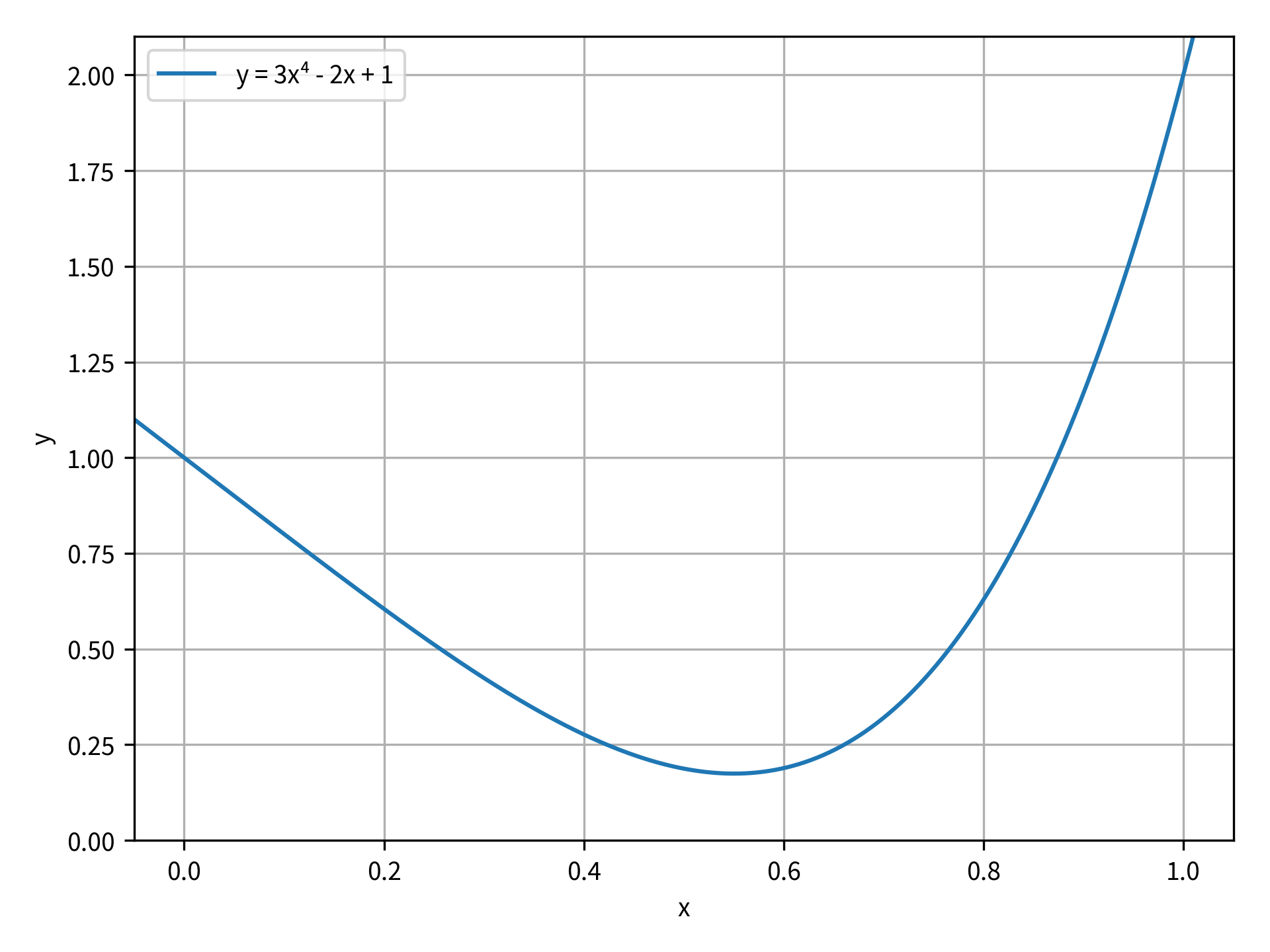
In the figure, you can see that there’s a minimum value of this function at approximately x = 0.55. You can use minimize_scalar() to determine the exact x and y coordinates of the minimum. First, import minimize_scalar() from scipy.optimize. Then, you need to define the objective function to be minimized:

Python
      
from scipy.optimize import minimize_scalar

def objective_function(x):
    return 3 * x ** 4 - 2 * x + 1

objective_function() takes the input x and applies the necessary mathematical operations to it, then returns the result. In the function definition, you can use any mathematical functions you want. The only limit is that the function must return a single number at the end.

Next, use minimize_scalar() to find the minimum value of this function. minimize_scalar() has only one required input, which is the name of the objective function definition:

Python
      
res = minimize_scalar(objective_function)

The output of minimize_scalar() is an instance of OptimizeResult. This class collects together many of the relevant details from the optimizer’s run, including whether or not the optimization was successful and, if successful, what the final result was. The output of minimize_scalar() for this function is shown below:

Text

     fun: 0.17451818777634331
    nfev: 16
     nit: 12
 success: True
       x: 0.5503212087491959

These results are all attributes of OptimizeResult. success is a Boolean value indicating whether or not the optimization completed successfully. If the optimization was successful, then fun is the value of the objective function at the optimal value x. You can see from the output that, as expected, the optimal value for this function was near x = 0.55.

Note: As you may know, not every function has a minimum. For instance, try and see what happens if your objective function is y = x³. For minimize_scalar(), objective functions with no minimum often result in an OverflowError because the optimizer eventually tries a number that is too big to be calculated by the computer.

On the opposite side of functions with no minimum are functions that have several minima. In these cases, minimize_scalar() is not guaranteed to find the global minimum of the function. However, minimize_scalar() has a method keyword argument that you can specify to control the solver that’s used for the optimization. The SciPy library has three built-in methods for scalar minimization:

brent is an implementation of Brent’s algorithm. This method is the default.
golden is an implementation of the golden-section search. The documentation notes that Brent’s method is usually better.
bounded is a bounded implementation of Brent’s algorithm. It’s useful to limit the search region when the minimum is in a known range.

When method is either brent or golden, minimize_scalar() takes another argument called bracket. This is a sequence of two or three elements that provide an initial guess for the bounds of the region with the minimum. However, these solvers do not guarantee that the minimum found will be within this range.

On the other hand, when method is bounded, minimize_scalar() takes another argument called bounds. This is a sequence of two elements that strictly bound the search region for the minimum. Try out the bounded method with the function y = x⁴ - x². This function is plotted in the figure below:

Using the previous example code, you can redefine objective_function() like so:

Python
      
    
def objective_function(x):
    return x ** 4 - x ** 2

First, try the default brent method:

Python
      
res = minimize_scalar(objective_function)

In this code, you didn’t pass a value for method, so minimize_scalar() used the brent method by default. The output is this:

Text

     fun: -0.24999999999999994
    nfev: 15
     nit: 11
 success: True
       x: 0.7071067853059209

You can see that the optimization was successful. It found the optimum near x = 0.707 and y = -1/4. If you solved for the minimum of the equation analytically, then you’d find the minimum at x = 1/√2, which is extremely close to the answer found by the minimization function. However, what if you wanted to find the symmetric minimum at x = -1/√2? You can return the same result by providing the bracket argument to the brent method:

Python
      
res = minimize_scalar(objective_function, bracket=(-1, 0))

In this code, you provide the sequence (-1, 0) to bracket to start the search in the region between -1 and 0. You expect there to be a minimum in this region since the objective function is symmetric about the y-axis. However, even with bracket, the brent method still returns the minimum at x = +1/√2. To find the minimum at x = -1/√2, you can use the bounded method with bounds:

Python
      
res = minimize_scalar(objective_function, method='bounded', bounds=(-1, 0))

In this code, you add method and bounds as arguments to minimize_scalar(), and you set bounds to be from -1 to 0. The output of this method is as follows:

Text

     fun: -0.24999999999998732
 message: 'Solution found.'
    nfev: 10
  status: 0
 success: True
       x: -0.707106701474177

As expected, the minimum was found at x = -1/√2. Note the additional output from this method, which includes a message attribute in res. This field is often used for more detailed output from some of the minimization solvers.

Remove ads

Minimizing a Function With Many Variables

scipy.optimize also includes the more general minimize(). This function can handle multivariate inputs and outputs and has more complicated optimization algorithms to be able to handle this. In addition, minimize() can handle constraints on the solution to your problem. You can specify three types of constraints:

LinearConstraint: The solution is constrained by taking the inner product of the solution x values with a user-input array and comparing the result to a lower and upper bound.
NonlinearConstraint: The solution is constrained by applying a user-supplied function to the solution x values and comparing the return value with a lower and upper bound.
Bounds: The solution x values are constrained to lie between a lower and upper bound.

When you use these constraints, it can limit the specific choice of optimization method that you’re able to use, since not all of the available methods support constraints in this way.

Let’s try a demonstration on how to use minimize(). Imagine you’re a stockbroker who’s interested in maximizing the total income from the sale of a fixed number of your stocks. You have identified a particular set of buyers, and for each buyer, you know the price they’ll pay and how much cash they have on hand.

You can phrase this problem as a constrained optimization problem. The objective function is that you want to maximize your income. However, minimize() finds the minimum value of a function, so you’ll need to multiply your objective function by -1 to find the x-values that produce the largest negative number.

There is one constraint on the problem, which is that the sum of the total shares purchased by the buyers does not exceed the number of shares you have on hand. There are also bounds on each of the solution variables because each buyer has an upper bound of cash available, and a lower bound of zero. Negative solution x-values mean that you’d be paying the buyers!

Try out the code below to solve this problem. First, import the modules you need and then set variables to determine the number of buyers in the market and the number of shares you want to sell:

Python
      
    
import numpy as np
from scipy.optimize import minimize, LinearConstraint

n_buyers = 10
n_shares = 15

In this code, you import numpy, minimize(), and LinearConstraint from scipy.optimize. Then, you set a market of 10 buyers who’ll be buying 15 shares in total from you.

Next, create arrays to store the price that each buyer pays, the maximum amount they can afford to spend, and the maximum number of shares each buyer can afford, given the first two arrays. For this example, you can use random number generation in np.random to generate the arrays:

Python
      
    
np.random.seed(10)
prices = np.random.random(n_buyers)
money_available = np.random.randint(1, 4, n_buyers)

In this code, you set the seed for NumPy’s random number generators. This function makes sure that each time you run this code, you’ll get the same set of random numbers. It’s here to make sure that your output is the same as the tutorial for comparison.

In line 7, you generate the array of prices the buyers will pay. np.random.random() creates an array of random numbers on the half-open interval [0, 1). The number of elements in the array is determined by the value of the argument, which in this case is the number of buyers.

In line 8, you generate an array of integers on the half-open interval from [1, 4), again with the size of the number of buyers. This array represents the total cash each buyer has available. Now, you need to compute the maximum number of shares each buyer can purchase:

Python
      
    
n_shares_per_buyer = money_available / prices
print(prices, money_available, n_shares_per_buyer, sep="\n")

In line 9, you take the ratio of the money_available with prices to determine the maximum number of shares each buyer can purchase. Finally, you print each of these arrays separated by a newline. The output is shown below:

Text

[0.77132064 0.02075195 0.63364823 0.74880388 0.49850701 0.22479665
 0.19806286 0.76053071 0.16911084 0.08833981]
[1 1 1 3 1 3 3 2 1 1]
[ 1.29647768 48.18824404  1.57816269  4.00638948  2.00598984 13.34539487
 15.14670609  2.62974258  5.91328161 11.3199242 ]

The first row is the array of prices, which are floating-point numbers between 0 and 1. This row is followed by the maximum cash available in integers from 1 to 4. Finally, you see the number of shares each buyer can purchase.

Now, you need to create the constraints and bounds for the solver. The constraint is that the sum of the total purchased shares can’t exceed the total number of shares available. This is a constraint rather than a bound because it involves more than one of the solution variables.

To represent this mathematically, you could say that x[0] + x[1] + ... + x[n] = n_shares, where n is the total number of buyers. More succinctly, you could take the dot or inner product of a vector of ones with the solution values, and constrain that to be equal to n_shares. Remember that LinearConstraint takes the dot product of the input array with the solution values and compares it to the lower and upper bound. You can use this to set up the constraint on n_shares:

Python
      
constraint = LinearConstraint(np.ones(n_buyers), lb=n_shares, ub=n_shares)

In this code, you create an array of ones with the length n_buyers and pass it as the first argument to LinearConstraint. Since LinearConstraint takes the dot product of the solution vector with this argument, it’ll result in the sum of the purchased shares.

This result is then constrained to lie between the other two arguments:

The lower bound lb
The upper bound ub

Since lb = ub = n_shares, this is an equality constraint because the sum of the values must be equal to both lb and ub. If lb were different from ub, then it would be an inequality constraint.

Next, create the bounds for the solution variable. The bounds limit the number of shares purchased to be 0 on the lower side and n_shares_per_buyer on the upper side. The format that minimize() expects for the bounds is a sequence of tuples of lower and upper bounds:

Python
      
bounds = [(0, n) for n in n_shares_per_buyer]

In this code, you use a comprehension to generate a list of tuples for each buyer. The last step before you run the optimization is to define the objective function. Recall that you’re trying to maximize your income. Equivalently, you want to make the negative of your income as large a negative number as possible.

The income that you generate from each sale is the price that the buyer pays multiplied by the number of shares they’re buying. Mathematically, you could write this as prices[0]*x[0] + prices[1]*x[1] + ... + prices[n]*x[n], where n is again the total number of buyers.

Once again, you can represent this more succinctly with the inner product, or x.dot(prices). This means that your objective function should take the current solution values x and the array of prices as arguments:

Python
      
    
def objective_function(x, prices):
    return -x.dot(prices)

In this code, you define objective_function() to take two arguments. Then you take the dot product of x with prices and return the negative of that value. Remember that you have to return the negative because you’re trying to make that number as small as possible, or as close to negative infinity as possible. Finally, you can call minimize():

Python
      
    
res = minimize(
    objective_function,
    x0=10 * np.random.random(n_buyers),
    args=(prices,),
    constraints=constraint,
    bounds=bounds,
)

In this code, res is an instance of OptimizeResult, just like with minimize_scalar(). As you’ll see, there are many of the same fields, even though the problem is quite different. In the call to minimize(), you pass five arguments:

objective_function: The first positional argument must be the function that you’re optimizing.
x0: The next argument is an initial guess for the values of the solution. In this case, you’re just providing a random array of values between 0 and 10, with the length of n_buyers. For some algorithms or some problems, choosing an appropriate initial guess may be important. However, for this example, it doesn’t seem too important.
args: The next argument is a tuple of other arguments that are necessary to be passed into the objective function. minimize() will always pass the current value of the solution x into the objective function, so this argument serves as a place to collect any other input necessary. In this example, you need to pass prices to objective_function(), so that goes here.
constraints: The next argument is a sequence of constraints on the problem. You’re passing the constraint you generated earlier on the number of available shares.
bounds: The last argument is the sequence of bounds on the solution variables that you generated earlier.

Once the solver runs, you should inspect res by printing it:

Text

     fun: -8.783020157087478
     jac: array([-0.7713207 , -0.02075195, -0.63364828, -0.74880385, 
       -0.49850702, -0.22479665, -0.1980629 , -0.76053071, -0.16911089,
       -0.08833981])
 message: 'Optimization terminated successfully.'
    nfev: 204
     nit: 17
    njev: 17
  status: 0
 success: True
       x: array([1.29647768e+00, 2.78286565e-13, 1.57816269e+00,
       4.00638948e+00, 2.00598984e+00, 3.48323773e+00, 3.19744231e-14,
       2.62974258e+00, 2.38121197e-14, 8.84962214e-14])

In this output, you can see message and status indicating the final state of the optimization. For this optimizer, a status of 0 means the optimization terminated successfully, which you can also see in the message. Since the optimization was successful, fun shows the value of the objective function at the optimized solution values. You’ll make an income of $8.78 from this sale.

You can see the values of x that optimize the function in res.x. In this case, the result is that you should sell about 1.3 shares to the first buyer, zero to the second buyer, 1.6 to the third buyer, 4.0 to the fourth, and so on.

You should also check and make sure that the constraints and bounds that you set are satisfied. You can do this with the following code:

Python
      
    
print("The total number of shares is:", sum(res.x))
print("Leftover money for each buyer:", money_available - res.x * prices)

In this code, you print the sum of the shares purchased by each buyer, which should be equal to n_shares. Then, you print the difference between each buyer’s cash on hand and the amount they spent. Each of these values should be positive. The output from these checks is shown below:

Text

The total number of shares is: 15.000000000000002
Leftover money for each buyer: [3.08642001e-14 1.00000000e+00 
 3.09752224e-14 6.48370246e-14 3.28626015e-14 2.21697984e+00
 3.00000000e+00 6.46149800e-14 1.00000000e+00 1.00000000e+00]

As you can see, all of the constraints and bounds on the solution were satisfied. Now you should try changing the problem so that the solver can’t find a solution. Change n_shares to a value of 1000, so that you’re trying to sell 1000 shares to these same buyers. When you run minimize(), you’ll find that the result is as shown below:

Text

     fun: nan
     jac: array([nan, nan, nan, nan, nan, nan, nan, nan, nan, nan])
 message: 'Iteration limit exceeded'
    nfev: 2182
     nit: 101
    njev: 100
  status: 9
 success: False
       x: array([nan, nan, nan, nan, nan, nan, nan, nan, nan, nan])

Notice that the status attribute now has a value of 9, and the message states that the iteration limit has been exceeded. There’s no way to sell 1000 shares given the amount of money each buyer has and the number of buyers in the market. However, rather than raising an error, minimize() still returns an OptimizeResult instance. You need to make sure to check the status code before proceeding with further calculations.

Remove ads

Conclusion

In this tutorial, you learned about the SciPy ecosystem and how that differs from the SciPy library. You read about some of the modules available in SciPy and learned how to install SciPy using Anaconda or pip. Then, you focused on some examples that use the clustering and optimization functionality in SciPy.

In the clustering example, you developed an algorithm to sort spam text messages from legitimate messages. Using kmeans(), you found that messages with more than about 20 digits are extremely likely to be spam!

In the optimization example, you first found the minimum value in a mathematically clear function with only one variable. Then, you solved the more complex problem of maximizing your profit from selling stocks. Using minimize(), you found the optimal number of stocks to sell to a group of buyers and made a profit of $8.79!

SciPy is a huge library, with many more modules to dive into. With the knowledge you have now, you’re well equipped to start exploring!

You can follow along with the examples in this tutorial by downloading the source code available at the link below:

Get Sample Code: Click here to get the sample code you’ll use to learn about SciPy in this tutorial.

What Do You Think?

Rate this article:

LinkedIn Twitter Facebook Email

What’s your #1 takeaway or favorite thing you learned? How are you going to put your newfound skills to use? Leave a comment below and let us know.

Commenting Tips: The most useful comments are those written with the goal of learning from or helping out other students. Get tips for asking good questions and get answers to common questions in our support portal.

Looking for a real-time conversation? Visit the Real Python Community Chat or join the next “Office Hours” Live Q&A Session. Happy Pythoning!

Scientific Python: Using SciPy for Optimization

Differentiating SciPy the Ecosystem and SciPy the Library

Understanding SciPy Modules

Installing SciPy on Your Computer

Anaconda

The pip Package Manager

Using the Cluster Module in SciPy

Using the Optimize Module in SciPy

Minimizing a Function With One Variable

Minimizing a Function With Many Variables

Conclusion

The `pip` Package Manager