Divide and Conquer Algorithms with Python Examples


Often I’ll hear about how you can optimise a for loop to be faster or how switch statements are faster than if statements. Most computers have over 1 core, with the ability to support multiple threads. Before worrying about optimising for loops or if statements try to attack your problem from a different angle.
Divide and Conquer is one way to attack a problem from a different angle. Don’t worry if you have zero experience or knowledge on the topic. This article is designed to be read by someone with very little programming knowledge.
I will explain this using 3 examples. The first will be a simple explanation. The second will be some code. The final will get into the mathematical core of divide and conquer techniques. (Don’t worry, I hate maths too).
What Is Divide and Conquer? 🌎
Divide and conquer is where you divide a large problem up into many smaller, much easier-to-solve problems. The rather small example below illustrates this.
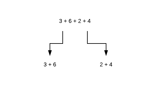
We take the equation “3 + 6 + 2 + 4” and cut it down into the smallest set of equations, which is [3 + 6, 2 + 4]. It could also be [2 + 3, 4 + 6]. The order doesn’t matter, as long as we turn this one long equation into many smaller equations.
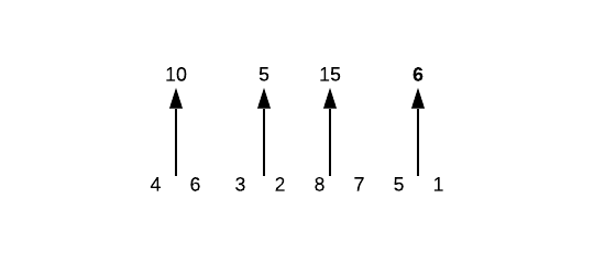
Let’s say we have 8 numbers:
We want to add them all together. We first divide the problem into 8 equal sub-problems. We do this by breaking the addition up into individual numbers.
We then add 2 numbers at a time.
Then 4 numbers into 8 numbers which is our resultant.
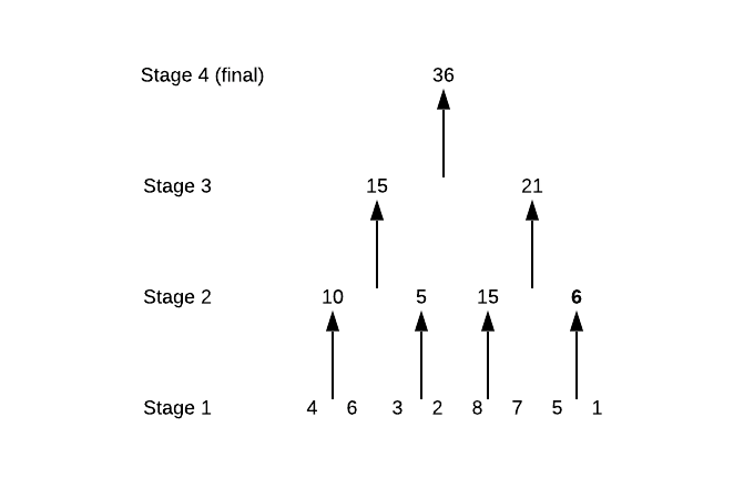
Why do we break it down to individual numbers at stage 1? Why don’t we just start from stage 2? Because while this list of numbers is even if the list was odd you would need to break it down to individual numbers to better handle it.
A divide and conquer algorithm tries to break a problem down into as many little chunks as possible since it is easier to solve with little chunks. It does this with recursion.
Recursion
Before we get into the rest of the article, let’s learn about recursion first.
Recursion is when a function calls itself. It’s a hard concept to understand if you’ve never heard of it before. This page provides a good explanation.
Matryoshka dolls are these cute little things:

We open up the bigger one and inside is a slightly smaller one. Inside that one is another slightly small doll. Let’s say, inside the last doll is a key. But we do not know how many dolls there are. How do we write a function that opens up the dolls until we find a key?
We could use a while loop, but recursion is preferred here.
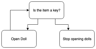
To program this, we can write:
def getKey(doll):
    item = doll.open()
    if item == key:
        return key
    else:
        return getKey(item)
getKey(doll)
The function repeatedly calls itself until it finds a key, at which point it stops. The finding key point is called a break case or exit condition.
We always add a break case to a recursive function. If we didn’t, it’d just be an infinite loop! Never-ending.
Computer scientists love recursion. Because it’s so hard for normal people to understand, we have a schadenfreude sensation watching people struggle. Haha just kidding!
We love recursion because it’s used in maths all the time. Computer scientists are mathematicians first, and coders second. Anything that brings code closer to real-life mathematics is good.
Not just because some people love maths, but because it makes it easier to implement. Need to calculate the Fibonacci numbers? The maths equation for this is:
A natural recurrence in our formula! Instead of translating it into loops, we can just calculate it:
def F(n):
    if n == 0 or n == 1:
        return n
    else:
        return F(n-1)+F(n-2)
This is one of the reasons why functional programming is so cool.
Also, as you’ll see throughout this article, recursion reads so much nicer than loops. And hey, maybe you can feel a little happier when your coworker doesn’t understand recursion but you do ;)
Back to Divide & Conquer
The technique, as defined in the famous Introduction to Algorithms by Cormen, Leiserson, Rivest, and Stein, is:
- Divide
If the problem is small, then solve it directly. Otherwise, divide the problem into smaller subsets of the same problem.
2. Conquer
Conquer the smaller problems by solving them recursively. If the sub-problems are small enough, recursion is not needed and you can solve them directly.
3. Combine
Take the solutions to the sub-problems and merge them into a solution to the original problem.
Let’s look at another example, calculating the factorial of a number.
n = 6

def recur_factorial(n):
    if n == 1:
        return n
    else:
        return n * recur_factorial(n-1)

print(recur_factorial(n))
With the code from above, some important things to note. The Divide part is also the recursion part. We divide the problem up at return n * recur_factorial(n-1).
The recur_factorial(n-1) part is where we divide the problem up.
The conquering part is the recursion part too, but also the if statement. If the problem is small enough, we solve it directly (by returning n). Else, we perform return n * recur_factorial(n-1).
Combine. We do this with the multiplication symbol. Eventually, we return the factorial of the number. If we didn’t have the symbol there, and it was return recur_factorial(n-1) it wouldn’t combine and it wouldn’t output anything similar to the factorial. (It’ll output 1, for those interested).
We’ll explore how to divide and conquer works in some famous algorithms, Merge Sort and the solution to the Towers of Hanoi.
One last time
- Divide / Break. Break the problem into smaller sub-problems.
- Conquer / Solve. Solves all the sub-problems.
- Merge / Combine. Merges all the sub-solutions into one solution.
Merge Sort 🤖
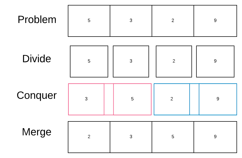
Merge Sort is a sorting algorithm. The algorithm works as follows:
- Divide the sequence of n numbers into 2 halves
- Recursively sort the two halves
- Merge the two sorted halves into a single sorted sequence
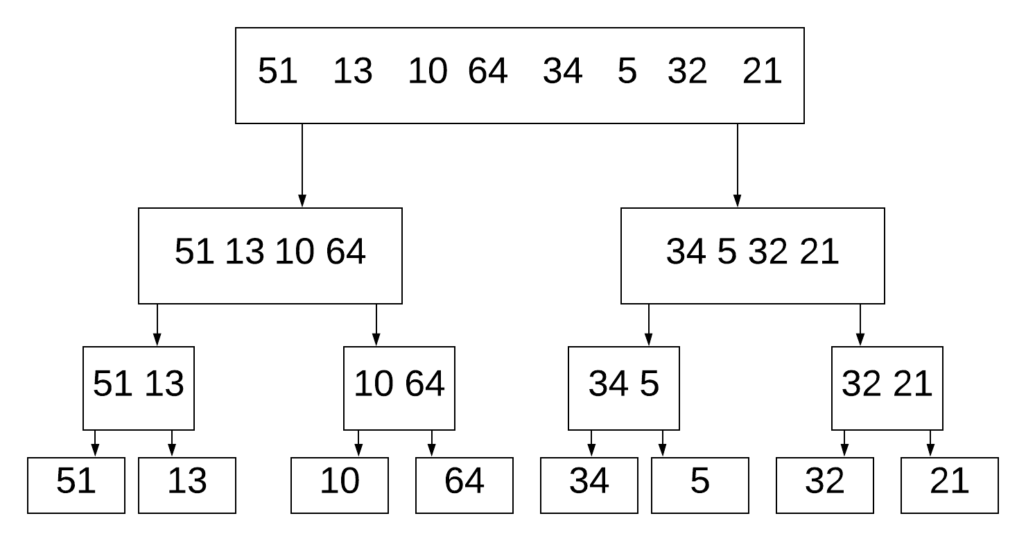
In this image, we break down the 8 numbers into separate digits. Just like we did earlier. Once we’ve done this, we can begin the sorting process.
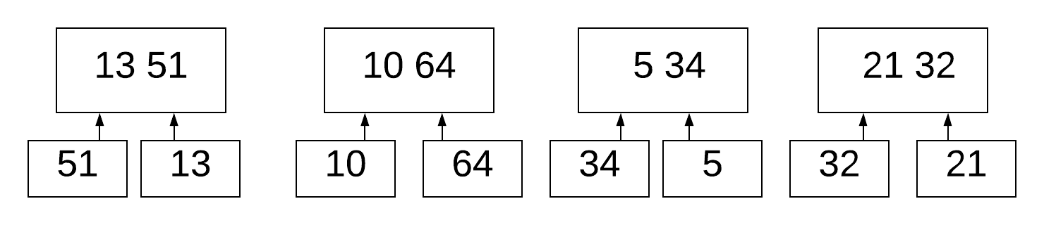
It compares 51 and 13. Since 13 is smaller, it puts it on the left-hand side. It does this for (10, 64), (34, 5), (32, 21).
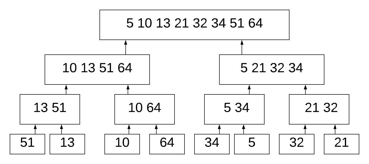
It then merges (13, 51) with (10, 64). It knows that 13 is the smallest in the first list, and 10 is the smallest in the right list. 10 is smaller than 13, therefore we don’t need to compare 13 to 64. We’re comparing & merging two **sorted **lists.
In recursion, we use the term base case to refer to the absolute smallest value we can deal with. With Merge Sort, the base case is 1. That means we split the list up until we get sub-lists of length 1. That’s also why we go down all the way to 1 and not 2. If the base case was 2, we would stop at the 2 numbers.
If the length of the list (n) is larger than 1, then we divide the list and each sub-list by 2 until we get sub-lists of size 1. If n = 1, the list is already sorted so we do nothing.
Merge Sort is an example of a divide-and-conquer algorithm. Let’s look at one more algorithm to understand how divide and conquer works.
Towers of Hanoi 🗼
The Towers of Hanoi is a mathematical problem which compromises 3 pegs and 3 discs. This problem is mostly used to teach recursion, but it has some real-world uses. The number of pegs & discs can change.
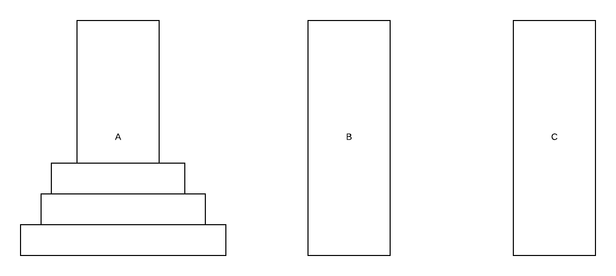
Each disc is a different size. We want to move all discs to peg C so that the largest is on the bottom, the second largest on top of the largest, third largest (smallest) on top of all of them. There are some rules to this game:
- We can only move 1 disc at a time.
- A disc cannot be placed on top of other discs that are smaller than it.
We want to use the smallest number of moves possible. If we have 1 disc, we only need to move it once. For 2 discs, we need to move it 3 times.
The number of moves is a power of 2 minus 1. Say we have 4 discs, we calculate the minimum number of moves as
To solve the above example we want to store the smallest disc in a buffer peg (1 move). See below for a gif on solving Tower of Hanoi with 3 pegs and 3 discs.

Notice how we need to have a buffer to store the discs.
We can generalise this problem. If we have n discs: move n-1 from A to B recursively, move largest from A to C, and move n-1 from B to C recursively.
If there is an even number of pieces the first move is always into the middle. If it is odd the first move is always to the other end.
Let’s code the algorithm for ToH, in pseudocode.
function MoveTower(disk, source, dest, spare):
    if disk == 0, then:
        move disk from source to dest
We start with a base case, disk == 0. source is the peg you’re starting at. dest is the final destination peg. spare is the spare peg.
FUNCTION MoveTower(disk, source, dest, spare):
IF disk == 0, THEN:
    move disk from source to dest
ELSE:
    MoveTower(disk - 1, source, spare, dest)   // Step 1
    move disk from source to dest              // Step 2
    MoveTower(disk - 1, spare, dest, source)   // Step 3
END IF
Notice that with step 1 we switch dest and source. We do not do this for step 3.
With recursion, we know 2 things:
- It always has a base case (if it doesn’t, how does the algorithm know to end?)
- The function calls itself.
The algorithm gets a little confusing with steps 1 and 3. They both call the same function. This is where multi-threading comes in. You can run steps 1 and 3 on different threads - at the same time.
Since 2 is more than 1, we move it down one more level again. So far you’ve seen what the divide and conquer technique is. You should understand how it works and what code looks like. Next, let’s learn how to define an algorithm to a problem using divide and conquer. This part is the most important. Once you know this, it’ll be easier to create divide and conquer algorithms.
How to identify Divide and Conquer problems
When we have a problem that looks similar to a famous divide & conquer algorithm (such as merge sort), it will be useful.
Most of the time, the algorithms we design will be most similar to merge sort. If we have an algorithm that takes a list and does something with each element of the list, it might be able to use divide & conquer.
For example, working out the largest item of a list. Given a list of words, how many times does the letter “e” appear?
If we have an algorithm that is slow and we would like to speed it up, one of our first options is divide and conquer.
There aren’t any obvious tell-tale signs other than “similar to a famous example”. But as we’ll see in the next section, we can check if it is solvable using divide & conquer.
How to solve problems using divide and conquer
Now we know how divide and conquer algorithms work, we can build up our own solution. In this example, we’ll walk through how to build a solution to the Fibonacci numbers.
Fibonacci Numbers 🐰
We can find Fibonacci numbers in nature. The way rabbits produce is in the style of the Fibonacci numbers. You have 2 rabbits that make 3, 3 rabbits make 5, 5 rabbits make 9 and so on.
The numbers start at 0 and the next number is the current number + the previous number. But by mathematical definition, the first 2 numbers are 0 and 1.
Let’s say we want to find the 5 Fibonacci numbers. We can do this:
# [0, 1]
0 + 1 = 1 # 3rd fib number
# [0, 1, 1]
1 + 1 = 2 # 4th fib number
# [0, 1, 1, 2]
2 + 1 = 3 # 5th fib number
# [0, 1, 1, 2, 3]
Now the first thing when designing a divide and conquer algorithm is to design the recurrence. The recurrence always starts with a base case.
We can describe this relation using a recursion. A recurrence is an equation which defines a function in terms of its smaller inputs. Recurrence and recursion sound similar and are similar.
As we saw, our base case is the 2 numbers at the start.
def f(n):
    if n == 0 or n == 1:
        return n
To calculate the 4th Fibonacci number, we do (4 - 1) + (4 - 2). This means (last number in the sequence) + (the number before the last). Or in other words:
The next number is the current number + the previous number.
If our number is not 0 or 1, we want to add the last 2 Fibonacci numbers together.
Let’s take a look at our table quickly:
# [0, 1]
0 + 1 = 1
# [0, 1, 1]
1 + 1 = 2
# [0, 1, 1, 2]
2 + 1 = 3
# [0, 1, 1, 2, 3]
2 + 3 = 5
# [0, 1, 1, 2, 3, 5]
But what if we don’t have this list stored? How do we calculate the 6th number without creating a list at all? Well we know that the 6th number is the 5th number + the 4th number. Okay, what are those? The 5th number is the 4th number + the 3rd number. The 4th number is the 3rd number + the second number.
We know that the second number is always 1, as we’ve reached a base case.

Eventually, we break it down to the base cases. Okay, so we know our code calls itself to calculate the Fibonacci numbers of the previous ones:
def f(n):
    if n == 0 or n == 1:
        return n
    else:
        f(n-1) f(n-2)
Okay, how do we merge the Fibonacci numbers at the end? As we saw, it is the last number **added **to the current number.
def f(n):
    if n == 0 or n == 1:
        return n
    else:
        f(n-1) + f(n-2)
Now we’ve seen this, let’s turn it into recursion using a recurrence. Luckily for us, it’s incredibly easy to go from a recurrence to code or from code to a recurrence, as they are both recurrences!
We often calculate the result of a recurrence using an execution tree. We saw this earlier when exploring how to build it in code. For F(6) this looks like:
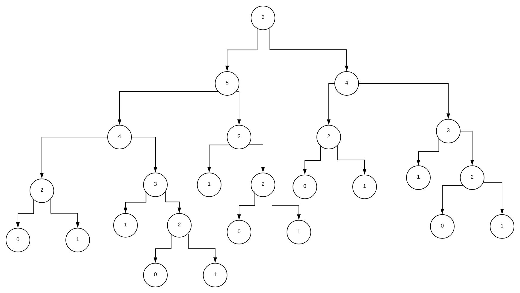
n is 4, and n is larger than 0 or 1. So we do f(n-1) + f(n-2). We ignore the addition for now. This results in 2 new nodes, 3 and 2. 3 is larger than 0 or 1 so we do the same. Same for 2. We do this until we get a bunch of nodes which are either 0 or 1.
We then add all the nodes together.
When Should I Use Divide & Conquer? 🎇
When we have a problem that looks similar to a famous divide & conquer algorithm (such as merge sort), it will be useful.
Most of the time, the algorithms we design will be most similar to merge sort. If we have an algorithm that takes a list and does something with each element of the list, it might be able to use divide & conquer.
For example, working out the largest item of a list. Given a list of words, how many times does the letter “e” appear?
Big O Notation of Divide & Conquer Algorithms
Normally if our algorithm follows a famous divide & conquer (algorithm) we can infer our big o from that.
This is no different from calculating the big o notation of our own algorithms.
Divide & Conquer vs Dynamic Programming vs Greedy
| Greedy vs Divide & Conquer vs Dynamic Programming | ||
|---|---|---|
| Greedy | Divide & Conquer | Dynamic Programming |
| Optimises by making the best choice at the moment | Optimises by breaking down a subproblem into simpler versions of itself and using multi-threading & recursion to solve | Same as Divide and Conquer, but optimises by caching the answers to each subproblem as not to repeat the calculation twice. |
| Doesn't always find the optimal solution, but is very fast | Always finds the optimal solution, but is slower than Greedy | Always finds the optimal solution, but could be pointless on small datasets. |
| Requires almost no memory | Requires some memory to remember recursive calls | Requires a lot of memory for memoisation / tabulation |
Conclusion 📕
Once you’ve identified how to break a problem down into many smaller pieces, you can use concurrent programming to execute these pieces at the same time (on different threads) speeding up the whole algorithm.
Divide-and-conquer algorithms are one of the fastest and perhaps easiest ways to increase the speed of an algorithm and are useful in everyday programming. Here are the most important topics we covered in this article:
- What is divide and conquer?
- Recursion
- Merge sort
- Towers of Hanoi
- Coding a divide and conquer algorithm
- Recurrences
- Fibonacci numbers
The next step is to explore multi-threading. Choose your programming language of choice and Google, as an example, “Python multi-threading”. Figure out how it works and see if you can attack any problems in your own code from this new angle.
You can also learn about how to solve recurrences (finding out the asymptotic running time of a recurrence), which is the next article I’m going to write. If you don’t want to miss it, or you liked this article do consider subscribing to my email list 😁