All You Need to Know About Big O Notation [Python Examples]

![All You Need to Know About Big O Notation [Python Examples]](https://images.unsplash.com/photo-1668902610778-96403019a7f5?crop=entropy&cs=tinysrgb&fit=max&fm=jpg&ixid=MnwxMTc3M3wwfDF8YWxsfDh8fHx8fHwyfHwxNjY5MTI5MTIx&ixlib=rb-4.0.3&q=80&w=2000)
By the end of this article, you’ll thoroughly understand Big O notation. You’ll also know how to use it in the real world, and even the mathematics behind it!
In computer science, time complexity is the computational complexity that describes the amount of time it takes to run an algorithm.
Big O notation is a method for determining how fast an algorithm is. Using Big O notation, we can learn whether our algorithm is fast or slow. This knowledge lets us design better algorithms.
This article is written using agnostic Python. That means it will be easy to port the Big O notation code over to Java, or any other language. If the code isn’t agnostic, there’s Java code accompanying it.
❓ How Do We Measure How Long an Algorithm Takes to Run?

We could run an algorithm 10,000 times and measure the average time taken.
➜ python3 -m timeit '[print(x) for x in range(100)]'
100 loops, best of 3: 11.1 msec per loop
➜ python3 -m timeit '[print(x) for x in range(10)]'
1000 loops, best of 3: 1.09 msec per loop
# We can see that the time per loop changes depending on the input!
Say we have an algorithm that takes a shopping list and prints out every item on the shopping list. If the shopping list has 3 items, it’ll execute quickly. If it has 10 billion items, it’ll take a long time.
What is the “perfect” input size to get the “perfect” measure of how long the algorithm takes?
Other things we need to consider:
- Different processor speeds exist.
- Languages matter. Assembly is faster than Scratch; how do we consider this?
For this reason, we use Big O (pronounced Big Oh) notation.
🤔 What Is Big O Notation?

Big O is a formal notation that describes the behaviour of a function when the argument tends towards the maximum input. It was invented by Paul Bachmann, Edmund Landau and others between 1894 and 1820s. Popularised in the 1970s by Donald Knuth. Big O takes the upper bound. The worst-case results in the worst execution of the algorithm. For our shopping list example, the worst-case is an infinite list.
Instead of saying the input is 10 billion, or infinite - we say the input is n size. The exact size of the input doesn’t matter, only how our algorithm performs with the worst input. We can still work out Big O without knowing the exact size of an input.
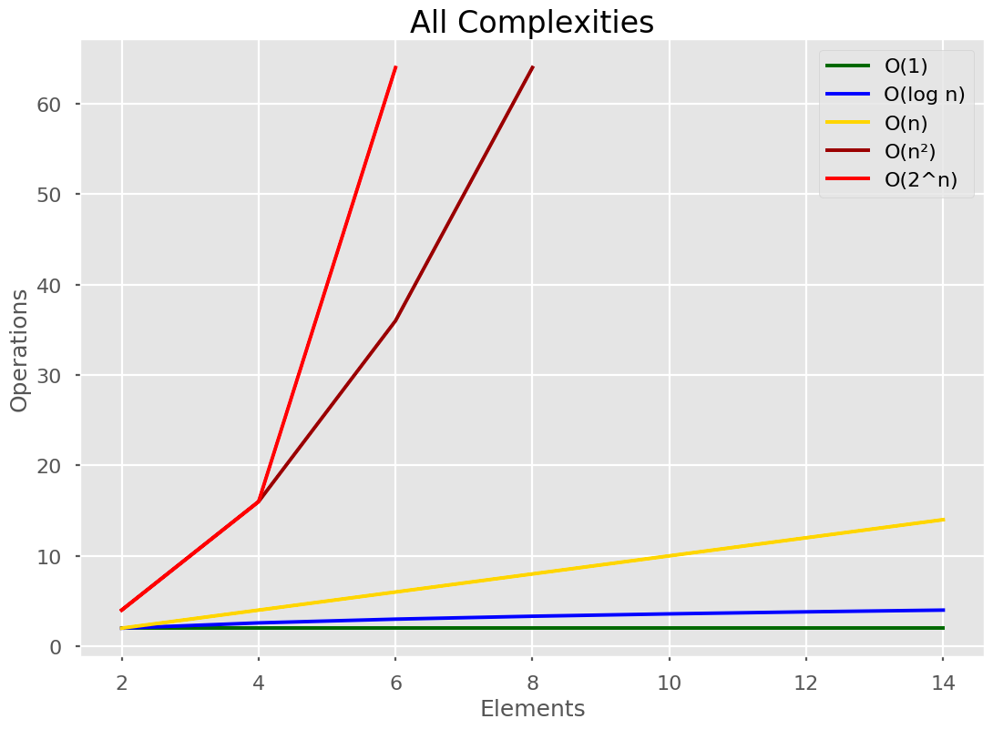
Big O is easy to read once we learn this table: The Big O Notation’s Order of Growth:
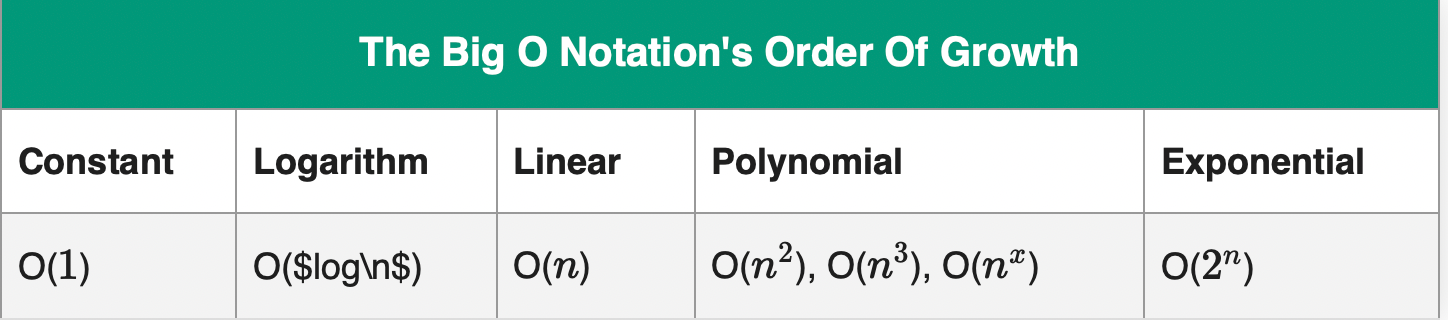
Where the further right they are, the longer it takes. n is the size of the input. Big O notation uses these functions to describe algorithm efficiency.
In our shopping list example, in the worst case of our algorithm, it prints out every item in the list sequentially. Since there are n items in the list, it takes O(n)O(n) polynomial time to complete the algorithm.
Other asymptotic (time-measuring) notations are:

Informally this is:
- Big Omega (best case)
- Big Theta (average case)
- Big O (worst case)
Let’s walk through every single column in our “The Big O Notation Table”.
🟢 Constant Time
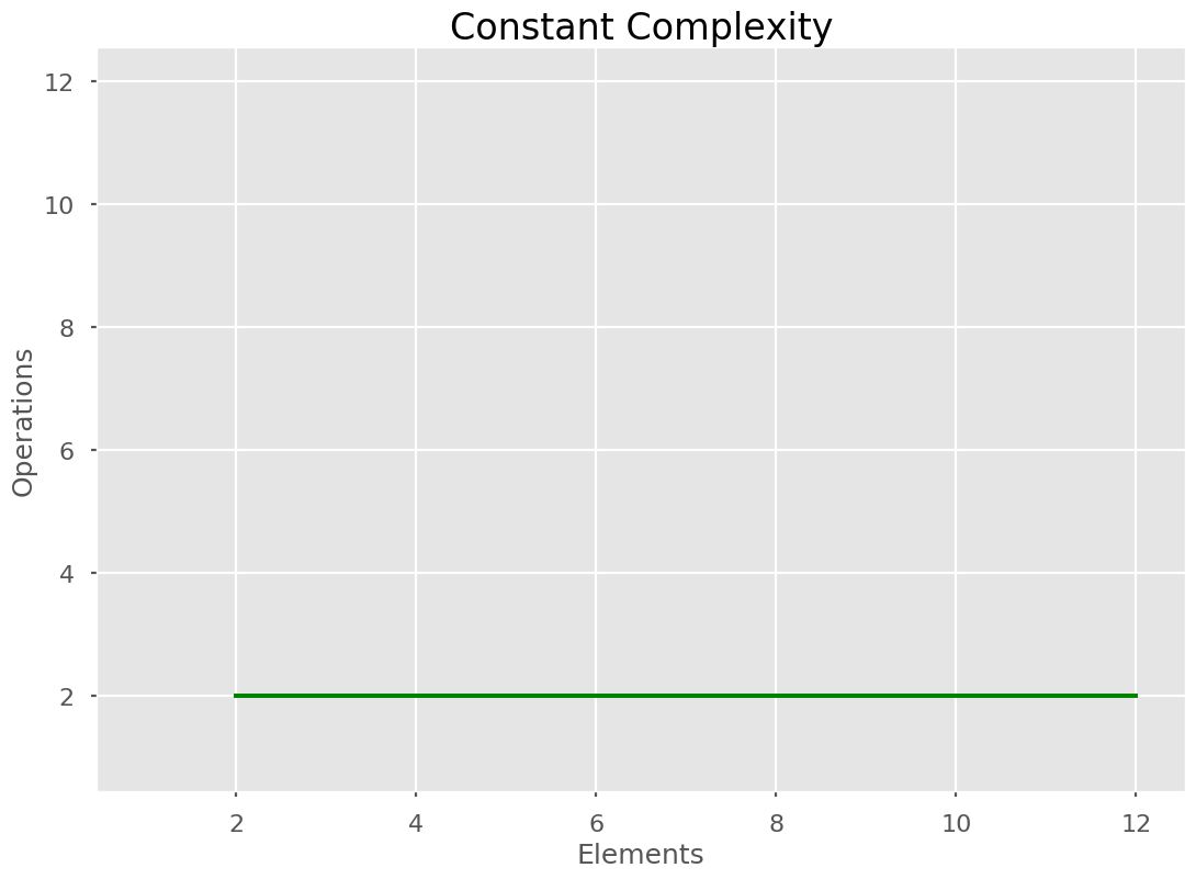
No matter how many elements, it will always take x operations to perform. In this case, 2. Constant algorithms do not scale with the input size, they are constant no matter how big the input. An example of this is addition. 1+2 takes the same time as 500+700. They may take more physical time, but we do not add more steps in the algorithm for the addition of big numbers. The underlying algorithm doesn’t change at all.
We often see constant as O(1), but any number could be used and it would still be constant. We sometimes change the number to a 1, because it doesn’t matter at all about how many steps it takes. What matters is that it takes a constant number of steps.
Constant time is the fastest of all Big O time complexities. The formal definition of constant time is:
It is upper-bounded by a constant
An example is:
def OddOrEven(n):
    return "Even" if n % 2 else "Odd"
Or in Java:
boolean isEven(double num) { return ((num % 2) == 0); }
In most programming languages, all integers have limits. Primitive operations (such as modulo, %) are all upper-bounded by this limit. If we go over this limit, we get an overflow error.
Because of this upper-bound, it satisfies O(1).
🔵 Logarithmic Time
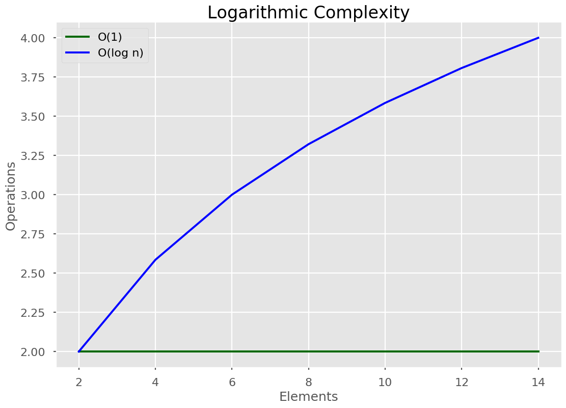
Here’s a quick explainer of what a logarithm is.
$$Log_{3}^{9}$$
What is being asked here is “3 to what power gives us 9?” This is 3 to the power of 2 gives us 9, so the whole expression looks like this:
$$Log_{3}^{9} = 2$$
A logarithmic algorithm halves the list every time it’s run.
Let’s look at binary search. Given the below-sorted list:
a = [1, 2, 3, 4, 5, 6 , 7, 8, 9, 10]
We want to find the number “2”.
We implement Binary Search as:
def binarySearch(alist, item):
    first = 0
    last = len(alist)-1
    found = False

    while first <= last and not found:
        midpoint = (first + last)//2
        if alist[midpoint] == item:
            found = True
        else:
            if item < alist[midpoint]:
            last = midpoint-1
            else:
                first = midpoint+1

    return found
In English, this is:
- Go to the middle of the list
- Check to see if that element is the answer
- If it’s not, check to see if that element is more than the item we want to find
- If it is, ignore the right-hand side (all the numbers higher than the midpoint) of the list and choose a new midpoint.
- Start over again, by finding the midpoint in the new list.
The algorithm halves the input every single time it iterates. Therefore it is logarithmic. Other examples include:
🟡 Linear Time
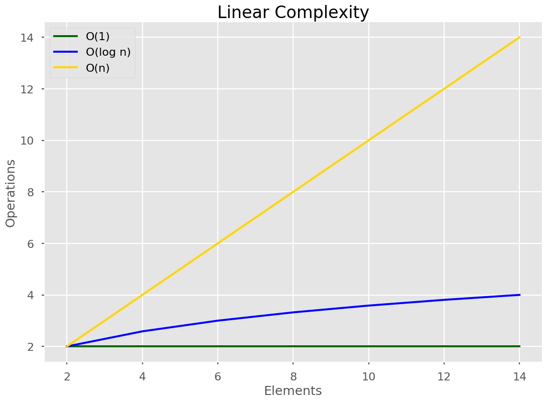
Linear time algorithms mean that every single element from the input is visited exactly once, O(n) times. As the size of the input, N, grows our algorithm’s run time scales exactly with the size of the input.
Linear running time algorithms are widespread. Linear runtime means that the program visits every element from the input. Linear time complexity O(n) means that as the input grows, the algorithms take proportionally longer to complete.2 Apr 2019
Remember our shopping list app from earlier? The algorithm ran in O(n) which is linear time!
Linear time is where every single item in a list is visited once, in a worst-case scenario.
To read out our shopping list, our algorithm has to read out each item. It can’t half the list, or add more items that we didn’t add. It has to list all n items, one at a time.
shopping_list = ["Bread", "Butter", "The Nacho Libre soundtrack from the 2006 film Nacho Libre", "Reusable Water Bottle"]
for item in shopping_list:
    print(item)
Let’s look at another example.
The largest item of an unsorted array
Given the list:
a = [2, 16, 7, 9, 8, 23, 12]
How do we work out what the largest item is?
We need to program it like this:
a = [2, 16, 7, 9, 8, 23, 12]
max_item = a[0]
for item in a:
    if item > max_item:
        max_item = item
We have to go through every item in the list, 1 by 1.
🔴 Polynomial Time
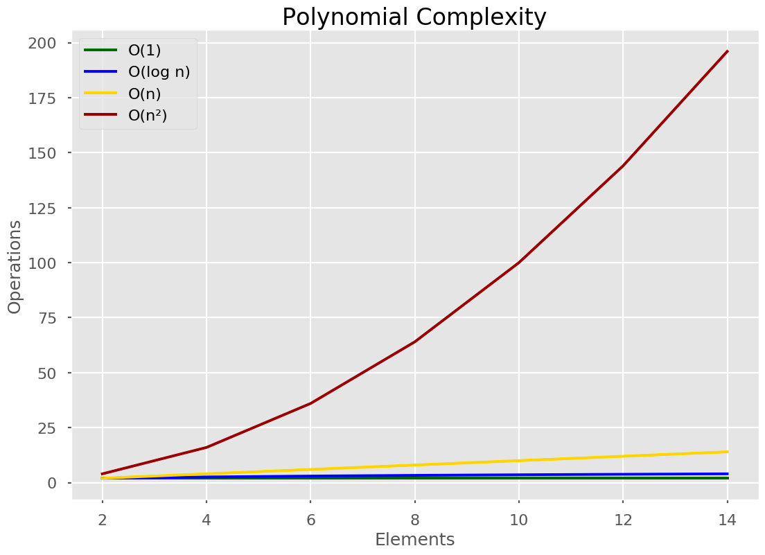
Notice how polynomial time dwarfs the others? Polynomial time is a polynomial function of the input. A polynomial function looks like n2 or n3 and so on.
If one loop through a list is O(n), 2 loops must be O(n2). For each loop, we go over the list once. For each item in that list, we go over the entire list once. Resulting in n2 operations.
a = [1, 2, 3, 4, 5, 6, 7, 8, 9, 10]
for i in a:
    for x in a:
        print("x")
For each nesting on the same list, that adds an extra +1 to the powers.
A triple nested loop is O(n3).
Bubblesort is a good example of anO(n2) algorithm. The sorting algorithm takes the first number and swaps it with the adjacent number if they are in the wrong order. It does this for each number until all numbers are in the right order - and thus sorted.
def bubbleSort(arr):
    n = len(arr)

    # Traverse through all array elements
    for i in range(n):

        # Last i elements are already in place
        for j in range(0, n-i-1):

            # traverse the array from 0 to n-i-1
            # Swap if the element found is greater
            # than the next element
            if arr[j] > arr[j+1] :
                arr[j], arr[j+1] = arr[j+1], arr[j]

# Driver code to test above
arr = [64, 34, 25, 12, 22, 11, 90]

bubbleSort(arr)
As a side note, my professor refers to any algorithm with a time of polynomial or above as:
A complete and utter disaster! This is a disaster! A catastrophe!
But the thing with large time complexities is that they often show us that something can be quickened.
For instance, a problem I had. Given a sentence, how many of those words appear in the English Dictionary? We can imagine the O(n2) method. One for loop through the sentence, another through the dictionary.
dictionary = ["a", "an"] # imagine if this was the dictionary
sentence = "hello uu988j my nadjjrjejas is brandon nanndwifjasj banana".split(" ")

counter = 0
for word in sentence:
    for item in dictionary:
        if word == item:
            counter = counter + 1
O(n2)! A disaster! But, knowing that this is a disaster means we can speed it up. Dictionaries are sorted by default. What if we sort our list of words in the sentence, and checked each word that way? We only need to loop through the dictionary once. And if the word we want to check is less than the word we’re on in the dictionary, we switch to the second word in the list.
Now our algorithm is O(n log n). We recognise that this isn’t a disaster, so we can move on! Knowing time complexities isn’t only useful in interviews. It’s an essential tool to improve our algorithms.
We can hasten many polynomial algorithms we construct using knowledge of algorithmic design.
❌ Exponential Time
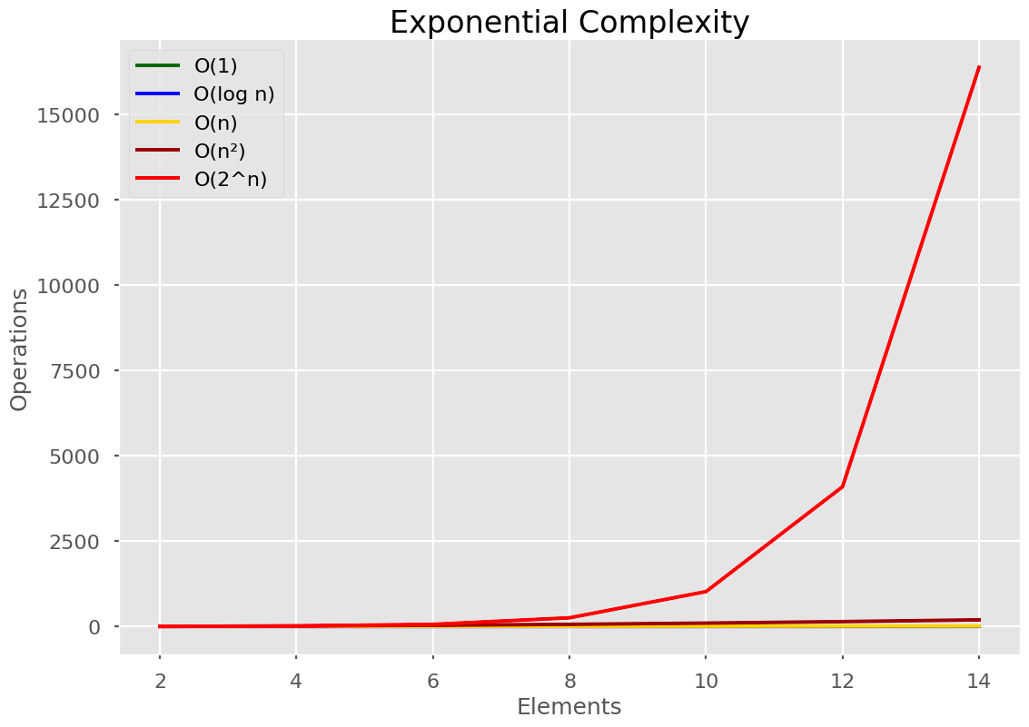
Exponential time is 2n, where 2 depends on the permutations involved.
This algorithm is the slowest of them all. You saw how my professor reacted to polynomial algorithms. He was jumping up and down in furiosity at exponential algorithms!
Say we have a password consisting only of numbers (so that’s 10 numbers, 0 through to 9). we want to crack a password which has a length of n, so to brute force through every combination we’ll have 10n combinations to work through.
One example of exponential time is to find all the subsets of a set.
>>> subsets([''])
['']
>>> subsets(['x'])
['', 'x']
>>> subsets(['a', 'b'])
['', 'a', 'b', 'ab']
We can see that when we have an input size of 2, the output size is 22=422=4.
Now, let’s code up subsets.
from itertools import chain, combinations

def subsets(iterable):
    s = list(iterable)
    return chain.from_iterable(combinations(s, r) for r in range(len(s)+1))
Taken from the documentation for itertools.
What’s important here is to see that it exponentially grows depending on the input size. Java code can be found here.
Exponential algorithms are horrific, but like polynomial algorithms we can learn a thing or two. Let’s say we have to calculate 104. We need to do this:
$$10 * 10 * 10 * 10 = 10^2 * 10^2$$
We have to calculate 102 twice! What if we store that value somewhere and use it later so we do not have to recalculate it? This is the principle of Dynamic Programming, which you can read about here.
When we see an exponential algorithm, dynamic programming can often be used to speed it up.
Again, knowing time complexities allows us to build better algorithms.
Here’s our Big O notation graph where the numbers are reduced so we can see all the different lines.
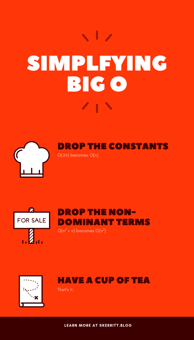
😌 Simplifying Big O notation

Rarely will time complexity be as easy as counting how many for loops we have. What if our algorithm looks like \(O(n+n2)\)? We can simplify our algorithm using these simple rules:
Drop the constants
If we have an algorithm described as O(2n), we drop the 2 so it becomes O(n).
Drop the non-dominant terms
O(n²+n) becomes O(n²). Only keep the larger one in Big O.
If we have a sum such as O(b²+a) we can’t drop either without knowledge of what b and a are.
Is that it?
Yup! The hardest part is figuring out what our program’s complexity is first. Simplifying is the easy part! Just remember the golden rule of Big O notation:
“What is the worst-case scenario here?”
☁ Other Big O Times to Learn (But Not Essential)
🥇 O(n log n)
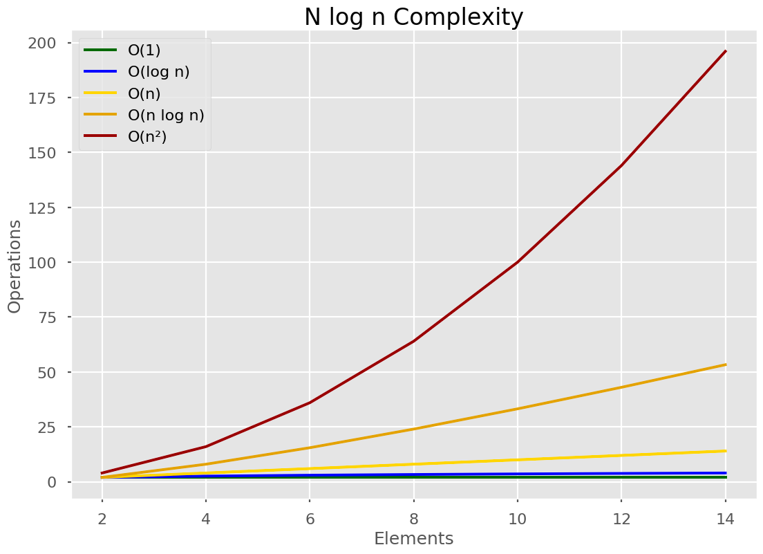
It falls between O(n) and O(n2). This is the fastest time possible for a comparison sort. We cannot get any faster unless we use some special property, like Radix sort. O(n log n) is the fastest comparison sort time.
It’s rather famous because Mergesort runs in O(n log n). Mergesort is a great algorithm not only because it sorts fast, but because the idea is used to build other algorithms.
Mergesort is used to teach divide & conquer algorithms. And for good reason, it’s a fantastic sorting algorithm that has roots outside of sorting.
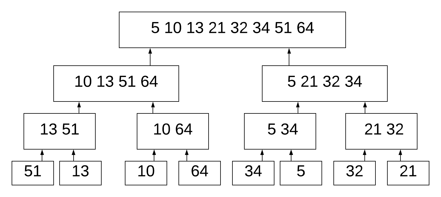
Mergesort works by breaking down the list of numbers into individual numbers:
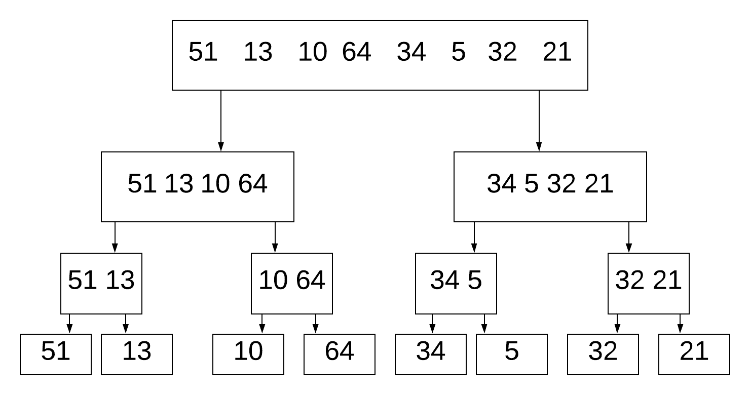
And then sorting each list, before merging them:
def mergeSort(alist):
    print("Splitting ",alist)
    if len(alist)>1:
        mid = len(alist)//2
        lefthalf = alist[:mid]
        righthalf = alist[mid:]

        mergeSort(lefthalf)
        mergeSort(righthalf)

        i=0
        j=0
        k=0
        while i < len(lefthalf) and j < len(righthalf):
            if lefthalf[i] <= righthalf[j]:
                alist[k]=lefthalf[i]
                i=i+1
            else:
                alist[k]=righthalf[j]
                j=j+1
            k=k+1

        while i < len(lefthalf):
            alist[k]=lefthalf[i]
            i=i+1
            k=k+1

        while j < len(righthalf):
            alist[k]=righthalf[j]
            j=j+1
            k=k+1
    print("Merging ",alist)

alist = [54,26,93,17,77,31,44,55,20]
mergeSort(alist)
print(alist)
👿 O(n!)
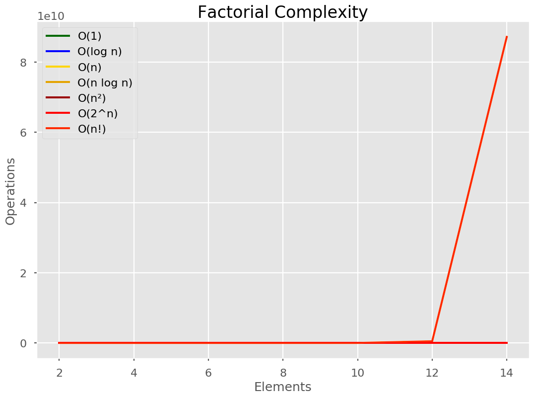
Notice the le10 at the top? This one is so large, it makes all other times look constant!
This time complexity is often used as a joke, referring to Bogo Sort. I have yet to find a real-life (not-a-joke) algorithm that runs in O(n!) that isn’t an algorithm calculating O(6!) or the likes.
🧮 How to Calculate Big O Notation for Our Own Algorithms with Examples

Our own algorithms will normally be based on some famous algorithm that already has a Big O notation. If it’s not, do not worry! Working out the Big O of our algorithm is easy.
Just think:
“What is the absolute worst input for my program?”
Take, for instance, a sequential searching algorithm.
def search(listInput, toFind):
    for counter, item in enumerate(listInput):
        if toFind == item:
            return (counter, item)
    return "did not find the item!"
The best input would be:
search(["apples"], "apples")
But the worst input is if the item was at the end of a long list.
search(["apples", "oranges", "The soundtrack from the 2006 film Nacho Libre", "Shrek"], "Shrek")
The worst-case scenario is O(n), because we have to go past every item in the list to find it.
What if our search algorithm was binary search? We learnt that binary search divides the list into half every time. This sounds like log n!
What if our binary search looks for an object, and then looks to find other similar objects?
# here we want to find the film shrek, find its IMDB rating and find other films with that IMDB rating. We are using binary search, then sequential search
toFind = {title: "Shrek", IMDBrating: None}
ret = search(toFind)
ret = search(ret['IMDBrating'])
We find Shrek with an IMDB score of 7.8. But we’re only sorted on the title, not the IMDB rating. We have to use a sequential search to find all other films with the same rating.
Binary search is O(log n) and sequential search is O(n), this makes our algorithm O(n log n). This isn’t a disaster, so we can be sure it’s not a terrible algorithm.
Even in instances where our algorithms are not strictly related to other algorithms, we can still compare them to things we know. O(log n) means halving. O(n2) means a nested for loop.
One last thing, we don’t always deal with n. Take this below algorithm:
x = [1, 2, 3, 4, 5]
y = [2, 6]
y = iter(y)
counter = 0
total = 0.0
while counter != len(x):
    # cycles through the y list.
    # multiplies 2 by 1, then 6 by 2. Then 2 by 3.
    total = total + x[counter] * next(y)
    counter += 1
print(total)
We have 2 inputs, x and y. Our notation is then O(x + y). Sometimes we cannot make our notation smaller without knowing more about the data.
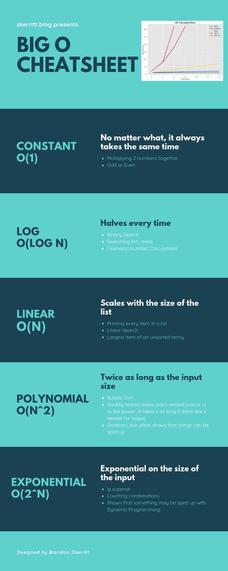
🤯 Big O Notation Cheat Sheet
I made this little infographic for you! The “add +1 for every nested for loop” depends on the for loop, as we saw earlier. But explaining that all over again would take up too much space 😅
🎓 How to Calculate Big O Notation of a Function (Discrete Maths)

Okay, this is where it gets hard. A lot of complaints against Big O notation is along the lines of:
“You didn’t really teach it, to really understand it you have to understand the maths!”
And I kinda agree. The surface-level knowledge above will be good for most interviews, but the stuff here is the stuff needed to master Big O notation.
Just as a reminder, we want to master asymptotic time complexity as it allows us to create better algorithms.
I’m going to be writing out the formal notation, and then explaining it simply. Over-simplification causes misinformation, so if you are studying for a test take your simplifications as generalities and not the truth. Mathematics is the whole truth, and you would be better off studying the maths rather than studying my simplifications. As I once read on the internet:
Shut up and calculate.
Is Big O Notation the Worst Case?
First things first, when I said:
Big O notation is the worst-case
That’s not true at all. It’s a white lie designed to help you learn the basics. Often used to get us to know enough to just pass interviews, but not enough to use it in the real world.
The formal definition of Big O notation is:
The upper-bounded time limit of the algorithm
Now, this often means “the worst-case” but not always. We can put upper bounds on whatever we want. But more often than not, we put upper bounds on the worst-case. In one of our examples, we’ll come across a weird formula where “the worst case” isn’t necessarily the one we choose for Big O.
This is an important distinction to make because some caveats will confuse us otherwise.
Given 2 positive functions, f(n) and g(n) we say f(n) is O(g(n)), written \(f(n) \in O(g(n))\), if there are constants c and n_0 such that:
$$f(n) \le c * g(n) \forall \geq n_o$$

Also, sometimes \(n_{0}\) is called k. But c stays the same.
This looks confusing but is just a fancy way of saying that the function (algorithm) is part of another function (the Big O notation used). Simplifying again: Our algorithm falls within the range of a Big O notation time complexity (O(n), O(log n), etc). So our algorithm is that time complexity (to simplify it).
Let’s see an example:
$$7n - 4 \in O(n)$$
Here we are claiming that 7n - 4 is in O(n) time. In formal Big O notation, we don't say it is that time. We say it falls within the range of that time.
We need to find constants c and n_0 such that \(7n-4 <= cn\) for all \(n >= n_{0}\). One choice is c = 7 and \(n_{o} = 1. 7 * 7 = 42 - 4 = 38\) and 7 * 1 = 7 so for all where n >= 7 this function holds true. This is just one of the many choices because any real number c >= 7 and any integer n_0 >= 1 would be okay. Another way to rephrase this is:
$$7n-4 \le 7n \; where \; n \geq 1$$
The left-hand side, 7n-4 is f(n). c = 10. g(n) = n. Therefore we can say f(n) =O(n) because g(n) = n. We say f(n) in O(n). All we have to do is substitute values into the formula until we find values for c and n that work. Let's do 10 examples now.
Example 1
$$f(n) = 4n^2 + 16n + 2$$
Is f(n) O(n4)?
We need to take this function:
$$f(n) = 4n^2 + 16n + 2$$
and say “is this less than some constant times n4?” We need to find out if there is such a constant.
$$n^2 + 16n + 2 \le n^4$$
Let’s do a chart. If n=0 we get:
$$0 + 0 + 2 = 2 \le 0$$
This isn’t true, so N = 0 is not true.
When n=1:
$$ 4 * 1 * 16 * 2 = 22 \le 1^4 = 22 \le 1$$
Is not true. Let’s try it again with n = 3.
$$50 \le 16$$
Not true, so let’s try another one. n=3.
$$86 \le 3^3 = 86 \le 81$$
Not true. Looks like the next one should work as we are approaching the tipping point. n=4.
$$ 130 \le 256$$
This is true. When n=4 or a greater number then this function where it’s less than N4 becomes True. When C=1, N≥4 this holds true.
The answer to the question “is this function, n2+16n+2n, Big O of n4 true?” Yes, when c=1 and n≥4.”
Note: I’m saying c=1 but I’m not writing \(c_n\) every time. Later on, using c will become important. But for these starter examples we’ll just assume c=1 until said otherwise.
Example 2
$$3n^2 + n + 16$$
Is this O(n2)?
We know that n <= n^2 for all n >= 1. Also, 16 <= n2 for n >= 4.
So:
$$3n^2 + n + 16 \le 3n^2 + n^2 + n^2 = 5n^2$$
for all n >= 4. The constant C is 5, and n_0 = 3.
Example 3
$$13n^3 + 7n \log \; n + 3$$
is O(n3)
Because log n >= n2 for all n >= 1, and for similar reasons as above we may conclude that: \(13n^3 + 6n ; n ; log ; n ; + 3 \le 21 n^3\) for all 'large enough' n. In this instance, c = 21.
Example 4
$$45n^5 - 10n^2 + 6n - 12$$
is O(n2)?
Any polynomial \(a_{k} n^k + ... + a_{2} n^2 + a_{1} n + a_{0}\) with \(a_{k} > 0\) is O(nk).
Along the same lines, we can argue that any polynomial \(a_{k} n^k + ... + a_2 n^2 + a_1 n + a-0\) with \(a_k > 0\) is also O(nj) for all j >= k. Therefore \(45n^5 - 10n^2 + 6n - 12\) is O(n2) (and is also O(n8) or O(n9) or O(nk) for any n >= 5).
Example 5
$$\sqrt{n}$$
is O(n)?
This doesn't hold true. \(\sqrt{n} = n^{1/2}\). Therefore \(O(n^{1/2}) < O(n)\). I hope you appreciate the easy example to break up the hard maths 😉
Example 6
$$ 3 \log_{n} + \log \log n$$
is O(log n)?
First we have this equality that \(log n <= n\) for every n >= 1. We can put a double log here like so: \(log log n <= log n\). Log log n is smaller than log n. We replaced "n" with "log n" on both sides of log n <= n. So:
$$3 \; log \; n + \; log \; log \; n \le 4 \; log \; n$$
So:
$$c = 4, n_0 = 1$$
Example 7
$$log \; n$$
is \(log \; n < O(\sqrt{n})\)
Log n grows slower than any function where this holds:
\(log \ m \le m^\epsilon\) for every \(\epsilon > 0\) no matter how small it is, as long as it is positive.
Using this inequality if we plug in \(\epsilon = \frac{1}{2}\) and we plug that into our equation \(\sqrt{m} = m^{\frac{1}{2}}\).
Knowing that \(log \ m \le m^\epsilon\) we know that \(O(log \ n) < O(\sqrt{n})\)
Example 8
$$2n + 3$$
What is the Big O of this?
$$2n + 3 \le 10n, n \geq 1$$
$$f(n) = O(n)$$.
This is because n is more than or equal to 1, it will always be larger than g(n) which is \(2n + 3\). Therefore, we have \(O(n)\).
Example 9
$$2n + 3 \le 10n$$
We don't have to write 10, it can be whatever we want so long as the equation holds true.
$$2n + 3 \le 2n + 3n$$
$$2n + 3 \le 5n, n \geq 1$$
Therefore \(f(n) = O(n)\).
Or we can write:
$$2n + 3 \le 5n^2 , n \geq 1$$
$$f(n) = 2n + 3$$
$$c = 5$$
$$g(n) = n^2$$
Can this same function be both \(O(n)\) and \(O(n^2)\)? Yes. It can be. This is where our definition of big o comes into play. It's the upper bound limit. We can say it is \(n^2, 2^n\) and any higher. But we cannot say it's lower.
When we write big o, we often want to use the closet function. Otherwise, we could say that every algorithm has an upper bound of \(O(2^n)\), which isn't true. Note: what we want to do (choose the closet function) is just a personal preference for most courses. All functions which work, which are the upper bound, are true.
There's a fantastic video on this strange concept here (and I took this example from there).
Summary
Big O represents how long an algorithm takes but sometimes we care about how much memory (space complexity) an algorithm takes too. If you're ever stuck, come back to this page and check out the infographics!