MATLAB® is widely known as a high-quality environment for any work that involves arrays, matrices, or linear algebra. Python is newer to this arena but is becoming increasingly popular for similar tasks. As you’ll see in this article, Python has all of the computational power of MATLAB for science tasks and makes it fast and easy to develop robust applications. However, there are some important differences when comparing MATLAB vs Python that you’ll need to learn about to effectively switch over.
In this article, you’ll learn how to:
- Evaluate the differences of using MATLAB vs Python
- Set up an environment for Python that duplicates the majority of MATLAB functions
- Convert scripts from MATLAB to Python
- Avoid common issues you might have when switching from MATLAB to Python
- Write code that looks and feels like Python
Free Bonus: Click here to get access to a free NumPy Resources Guide that points you to the best tutorials, videos, and books for improving your NumPy skills.
MATLAB vs Python: Comparing Features and Philosophy
Python is a high-level, general-purpose programming language designed for ease of use by human beings accomplishing all sorts of tasks. Python was created by Guido van Rossum and first released in the early 1990s. Python is a mature language developed by hundreds of collaborators around the world.
Python is used by developers working on small, personal projects all the way up to some of the largest internet companies in the world. Not only does Python run Reddit and Dropbox, but the original Google algorithm was written in Python. Also, the Python-based Django Framework runs Instagram and many other websites. On the science and engineering side, the data to create the 2019 photo of a black hole was processed in Python, and major companies like Netflix use Python in their data analytics work.
There is also an important philosophical difference in the MATLAB vs Python comparison. MATLAB is proprietary, closed-source software. For most people, a license to use MATLAB is quite expensive, which means that if you have code in MATLAB, then only people who can afford a license will be able to run it. Plus, users are charged for each additional toolbox they want to install to extend the basic functionality of MATLAB. Aside from the cost, the MATLAB language is developed exclusively by Mathworks. If Mathworks were ever to go out of business, then MATLAB would no longer be able to be developed and might eventually stop functioning.
On the other hand, Python is free and open-source software. Not only can you download Python at no cost, but you can also download, look at, and modify the source code as well. This is a big advantage for Python because it means that anyone can pick up the development of the language if the current developers were unable to continue for some reason.
If you’re a researcher or scientist, then using open-source software has some pretty big benefits. Paul Romer, the 2018 Nobel Laureate in Economics, is a recent convert to Python. By his estimation, switching to open-source software in general, and Python in particular, brought greater integrity and accountability to his research. This was because all of the code could be shared and run by any interested reader. Prof. Romer wrote an excellent article, Jupyter, Mathematica, and the Future of the Research Paper, about his experience with open-source software.
Moreover, since Python is available at no cost, a much broader audience can use the code you develop. As you’ll see a little later on in the article, Python has an awesome community that can help you get started with the language and advance your knowledge. There are tens of thousands of tutorials, articles, and books all about Python software development. Here are a few to get you started:
Plus, with so many developers in the community, there are hundreds of thousands of free packages to accomplish many of the tasks that you’ll want to do with Python. You’ll learn more about how to get these packages later on in this article.
Like MATLAB, Python is an interpreted language. This means that Python code can be ported between all of the major operating system platforms and CPU architectures out there, with only small changes required for different platforms. There are distributions of Python for desktop and laptop CPUs and microcontrollers like Adafruit. Python can also talk to other microcontrollers like Arduino with a simple programming interface that is almost identical no matter the host operating system.
For all of these reasons, and many more, Python is an excellent choice to replace MATLAB as your programming language of choice. Now that you’re convinced to try out Python, read on to find out how to get it on your computer and how to switch from MATLAB!
Note: GNU Octave is a free and open-source clone of MATLAB. In this sense, GNU Octave has the same philosophical advantages that Python has around code reproducibility and access to the software.
Octave’s syntax is mostly compatible with MATLAB syntax, so it provides a short learning curve for MATLAB developers who want to use open-source software. However, Octave can’t match Python’s community or the number of different kinds of applications that Python can serve, so we definitely recommend you switch whole hog over to Python.
Besides, this website is called Real Python, not Real Octave 😀
Setting Up Your Environment for Python
In this section, you’ll learn:
- How to install Python on your computer for a seamless transition from MATLAB
- How to install replacements for the MATLAB integrated development environment
- How to use the replacements for MATLAB on your computer
Getting Python via Anaconda
Python can be downloaded from a number of different sources, called distributions. For instance, the Python that you can download from the official Python website is one distribution. Another very popular Python distribution, particularly for math, science, engineering, and data science applications, is the Anaconda distribution.
There are two main reasons that Anaconda is so popular:
-
Anaconda distributes pre-built packages for Windows, macOS, and Linux, which means that the installation process is really easy and the same for all three major platforms.
-
Anaconda includes all of the most popular packages for engineering and data science type workloads in one single installer.
For the purposes of creating an environment that is very similar to MATLAB, you should download and install Anaconda. As of this writing, there are two major versions of Python available: Python 2 and Python 3. You should definitely install the version of Anaconda for Python 3, since Python 2 will not be supported past January 1, 2020. Python 3.7 is the most recent version at the time of this writing, but Python 3.8 should be out a few months after this article is published. Either 3.7 or 3.8 will work the same for you, so choose the most recent version you can.
Once you have downloaded the Anaconda installer, you can follow the default set up procedures depending on your platform. You should install Anaconda in a directory that does not require administrator permission to modify, which is the default setting in the installer.
With Anaconda installed, there are a few specific programs you should know about. The easiest way to launch applications is to use the Anaconda Navigator. On Windows, you can find this in the Start Menu and on macOS you can find it in Launchpad. Here’s a screenshot of the Anaconda Navigator on Windows:

In the screenshot, you can see several installed applications, including JupyterLab, Jupyter Notebook, and Spyder, that you’ll learn more about later in this tutorial.
On Windows, there is one other application that you should know about. This is called Anaconda Prompt, and it is a command prompt set up specifically to work with conda on Windows. If you want to type conda commands in a terminal, rather than using the Navigator GUI, then you should use Anaconda Prompt on Windows.
On macOS, you can use any terminal application such as the default Terminal.app or iTerm2 to access conda from the command line. On Linux, you can use the terminal emulator of your choice and which specific emulator is installed will depend on your Linux distribution.
Terminology Note: You may be a little bit confused about conda versus Anaconda. The distinction is subtle but important. Anaconda is a distribution of Python that includes many of the necessary packages for scientific work of all kinds. conda is a cross-platform package management software that is included with the Anaconda distribution of Python. conda is the software that you use to build, install, and remove packages within the Anaconda distribution.
You can read all about how to use conda in Setting Up Python for Machine Learning on Windows. Although that tutorial focuses on Windows, the conda commands are the same on Windows, macOS, and Linux.
Python also includes another way to install packages, called pip. If you’re using Anaconda, you should always prefer to install packages using conda whenever possible. Sometimes, though, a package is only available with pip, and for those cases, you can read What Is Pip? A Guide for New Pythonistas.
Getting an Integrated Development Environment
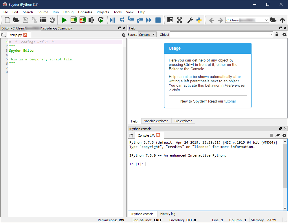
One of the big advantages of MATLAB is that it includes a development environment with the software. This is the window that you’re most likely used to working in. There is a console in the center where you can type commands, a variable explorer on the right, and a directory listing on the left.
Unlike MATLAB, Python itself does not have a default development environment. It is up to each user to find one that fits their needs. Fortunately, Anaconda comes with two different integrated development environments (IDEs) that are similar to the MATLAB IDE to make your switch seamless. These are called Spyder and JupyterLab. In the next two sections, you’ll see a detailed introduction to Spyder and a brief overview of JupyterLab.
Spyder
Spyder is an IDE for Python that is developed specifically for scientific Python work. One of the really nice things about Spyder is that it has a mode specifically designed for people like you who are converting from MATLAB to Python. You’ll see that a little later on.
First, you should open Spyder. If you followed the instructions in the previous section, you can open Spyder using the Anaconda Navigator. Just find the Spyder icon and click the Launch button. You can also launch Spyder from the Start Menu if you’re using Windows or from Launchpad if you’re using macOS.
Changing the Default Window Layout in Spyder
The default window in Spyder looks like the image below. This is for version 3.3.4 of Spyder running on Windows 10. It should look quite similar on macOS or Linux:
Before you take a tour of the user interface, you can make the interface look a little more like MATLAB. In the View → Window layouts menu choose MATLAB layout. That will change the window automatically so it has the same areas that you’re used to from MATLAB, annotated on the figure below:
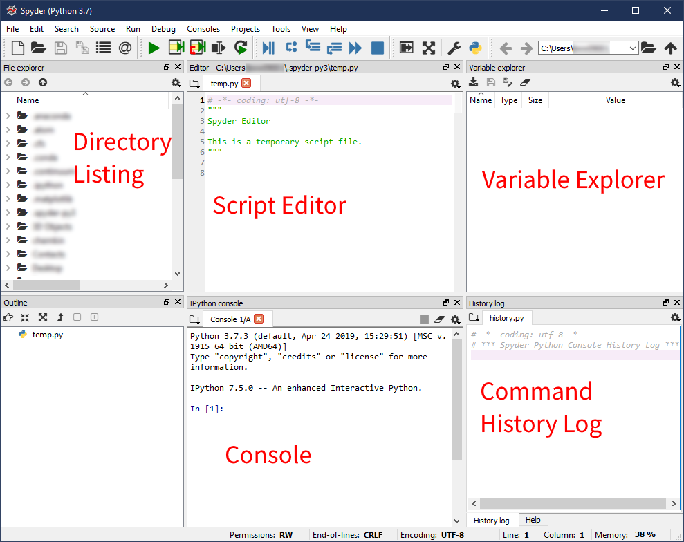
In the top left of the window is the File Explorer or directory listing. In this pane, you can find files that you want to edit or create new files and folders to work with.
In the top center is a file editor. In this editor, you can work on Python scripts that you want to save to re-run later on. By default, the editor opens a file called temp.py located in Spyder’s configuration directory. This file is meant as a temporary place to try things out before you save them in a file somewhere else on your computer.
In the bottom center is the console. Like in MATLAB, the console is where you can run commands to see what they do or when you want to debug some code. Variables created in the console are not saved if you close Spyder and open it up again. The console is technically running IPython by default.
Any commands that you type in the console will be logged into the history file in the bottom right pane of the window. Furthermore, any variables that you create in the console will be shown in the variable explorer in the top right pane.
Notice that you can adjust the size of any pane by putting your mouse over the divider between panes, clicking, and dragging the edge to the size that you want. You can close any of the panes by clicking the x in the top of the pane.
You can also break any pane out of the main window by clicking the button that looks like two windows in the top of the pane, right next to the x that closes the pane. When a pane is broken out of the main window, you can drag it around and rearrange it however you want. If you want to put the pane back in the main window, drag it with the mouse so a transparent blue or gray background appears and the neighboring panes resize, then let go and the pane will snap into place.
Once you have the panes arranged exactly how you want, you can ask Spyder to save the layout. Go to the View menu and find the Window layouts flyout again. Then click Save current layout and give it a name. This lets you reset to your preferred layout at any time if something gets changed by accident. You can also reset to one of the default configurations from this menu.
Running Statements in the Console in Spyder
In this section, you’re going to be writing some simple Python commands, but don’t worry if you don’t quite understand what they mean yet. You’ll learn more about Python syntax a little later on in this article. What you want to do right now is get a sense for how Spyder’s interface is similar to and different from the MATLAB interface.
You’ll be working a lot with the Spyder console in this article, so you should learn about how it works. In the console, you’ll see a line that starts with In [1]:, for input line 1. Spyder (really, the IPython console) numbers all of the input lines that you type. Since this is the first input you’re typing, the line number is 1. In the rest of this article, you’ll see references to “input line X,” where X is the number in the square brackets.
One of the first things I like to do with folks who are new to Python is show them the Zen of Python. This short poem gives you a sense of what Python is all about and how to approach working with Python.
To see the Zen of Python, type import this on input line 1 and then run the code by pressing Enter. You’ll see an output like below:
In [1]: import this
The Zen of Python, by Tim Peters

Beautiful is better than ugly.
Explicit is better than implicit.
Simple is better than complex.
Complex is better than complicated.
Flat is better than nested.
Sparse is better than dense.
Readability counts.
Special cases aren't special enough to break the rules.
Although practicality beats purity.
Errors should never pass silently.
Unless explicitly silenced.
In the face of ambiguity, refuse the temptation to guess.
There should be one-- and preferably only one --obvious way to do it.
Although that way may not be obvious at first unless you're Dutch.
Now is better than never.
Although never is often better than *right* now.
If the implementation is hard to explain, it's a bad idea.
If the implementation is easy to explain, it may be a good idea.
Namespaces are one honking great idea -- let's do more of those!
This code has import this on input line 1. The output from running import this is to print the Zen of Python onto the console. We’ll return to several of the stanzas in this poem later on in the article.
In many of the code blocks in this article, you’ll see three greater-than signs (>>>) in the top right of the code block. If you click that, it will remove the input prompt and any output lines, so you can copy and paste the code right into your console.
Many Pythonistas maintain a healthy sense of humor. This is displayed in many places throughout the language, including the Zen of Python. For another one, in the Spyder console, type the following code, followed by Enter to run it:
In [2]: import antigravity
That statement will open your web browser to the webcomic called XKCD, specifically comic #353, where the author has discovered that Python has given him the ability to fly!
You’ve now successfully run your first two Python statements! Congratulations 😃🎉
If you look at the History Log, you should see the first two commands you typed in the console (import this and import antigravity). Let’s define some variables and do some basic arithmetic now. In the console, type the following statements, pressing Enter after each one:
In [3]: var_1 = 10
In [4]: var_2 = 20
In [5]: var_3 = var_1 + var_2
In [6]: var_3
Out[6]: 30
In this code, you defined 3 variables: var_1, var_2, and var_3. You assigned var_1 the value 10, var_2 the value 20, and var_3 the sum of var_1 and var_2. Then you showed the value of the var_3 variable by writing it as the only thing on the input line. The output from that statement is shown on the next Out line, and the number on the Out line matches the associated In line.
There are two main things for you to notice in these commands:
-
If a statement does not include an assignment (with an
=), it is printed onto anOutline. In MATLAB, you would need to include a semicolon to suppress the output even from assignment statements, but that is not necessary in Python. -
On input lines 3, 4, and 5, the Variable explorer in the top right pane updated.
After you run these three commands, your Variable explorer should look like the image below:
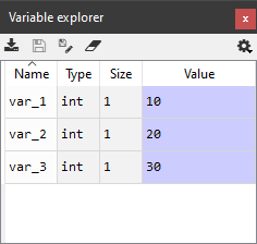
In this image, you can see a table with four columns:
- Name shows the name that you gave to
var_1,var_2, andvar_3. - Type shows the Python type of the variable, in this case, all
intfor integer numbers. - Size shows the size of the data stored variable, which is more useful for lists and other data structures.
- Value shows the current value of the variable.
Running Code in Files in Spyder
The last stop in our brief tour of the Spyder interface is the File editor pane. In this pane, you can create and edit Python scripts and run them using the console. By default, Spyder creates a temporary file called temp.py which is intended for you to temporarily store commands as you’re working before you move or save them in another file.
Let’s write some code into the temp.py file and see how to run it. The file starts with the following code, which you can just leave in place:
 1# -*- coding: utf-8 -*-
 2"""
 3Spyder Editor
 4
 5This is a temporary script file.
 6"""
In this code, you can see two Python syntax structures:
-
Line 1 has a comment. In Python, the comment character is the hash or pound sign (
#). MATLAB uses the percent symbol (%) as the comment character. Anything following the hash on the line is a comment and is usually ignored by the Python interpreter. -
Starting on line 2 is a string that provides some context for the contents of the file. This is often referred to as a documentation string or docstring for short. You’ll learn more about docstrings in a later section.
Now you can start adding code to this file. Starting on line 8 in temp.py, enter the following code that is similar to what you already typed in the console:
 8var_4 = 10
 9var_5 = 20
10var_6 = var_4 + var_5
Then, there are three ways to run the code:
- You can use the F5 keyboard shortcut to run the file just like in MATLAB.
- You can click the green right-facing triangle in the menu bar just above the Editor and File explorer panes.
- You can use the Run → Run menu option.
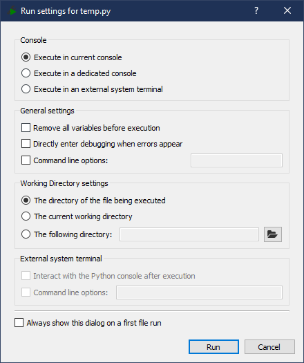
The first time you run a file, Spyder will open a dialog window asking you to confirm the options you want to use. For this test, the default options are fine and you can click Run at the bottom of the dialog box:
This will automatically execute the following code in the console:
In [7]: runfile('C:/Users/Eleanor/.spyder-py3/temp.py',
   ...:         wdir='C:/Users/Eleanor/.spyder-py3')
This code will run the file that you were working on. Notice that running the file added three variables into the Variable explorer: var_4, var_5, and var_6. These are the three variables that you defined in the file. You will also see runfile() added to the History log.
In Spyder, you can also create code cells that can be run individually. To create a code cell, add a line that starts with # %% into the file open in the editor:
11# %% This is a code cell
12var_7 = 42
13var_8 = var_7 * 2
14
15# %% This is a second code cell
16print("This code will be executed in this cell")
In this code, you have created your first code cell on line 11 with the # %% code. What follows is a line comment and is ignored by Python. On line 12, you are assigning var_7 to have the value 42 and then line 13 assigns var_8 to be var_7 times two. Line 15 starts another code cell that can be executed separately from the first one.
To execute the code cells, click the Run Current Cell or Run Current Cell and Go to the Next One buttons next to the generic Run button in the toolbar. You can also use the keyboard shortcuts Ctrl+Enter to run the current cell and leave it selected, or Shift+Enter to run the current cell and select the next cell.
Spyder also offers easy-to-use debugging features, just like in MATLAB. You can double-click any of the line numbers in the Editor to set a breakpoint in your code. You can run the code in debug mode using the blue right-facing triangle with two vertical lines from the toolbar, or the Ctrl+F5 keyboard shortcut. This will pause execution at any breakpoints you specify and open the ipdb debugger in the console which is an IPython-enhanced way to run the Python debugger pdb. You can read more in Python Debugging With pdb.
Summarizing Your Experience in Spyder
Now you have the basic tools to use Spyder as a replacement for the MATLAB integrated development environment. You know how to run code in the console or type code into a file and run the file. You also know where to look to see your directories and files, the variables that you’ve defined, and the history of the commands you typed.
Once you’re ready to start organizing your code into modules and packages, you can check out the following resources:
- Python Modules and Packages – An Introduction
- How to Publish an Open-Source Python Package to PyPI
- How to Publish Your Own Python Package to PyPI
Spyder is a really big piece of software, and you’ve only just scratched the surface. You can learn a lot more about Spyder by reading the official documentation, the troubleshooting and FAQ guide, and the Spyder wiki.
JupyterLab
JupyterLab is an IDE developed by Project Jupyter. You may have heard of Jupyter Notebooks, particularly if you’re a data scientist. Well, JupyterLab is the next iteration of the Jupyter Notebook. Although at the time of this writing JupyterLab is still in beta, Project Jupyter expects that JupyterLab will eventually replace the current Notebook server interface. However, JupyterLab is fully compatible with existing Notebooks so the transition should be fairly seamless.
JupyterLab comes preinstalled with Anaconda, so you can launch it from the Anaconda Navigator. Find the JupyterLab box and click Launch. This will open your web browser to the address http://localhost:8888/lab.
The main JupyterLab window is shown in the picture below:
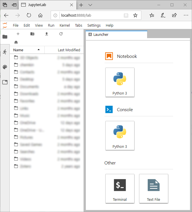
There are two main sections of the interface:
- On the left is a File explorer that lets you open files from your computer.
- On the right side of the window is how you can open create new Notebook files, work in an IPython console or system terminal, or create a new text file.
If you’re interested in learning more about JupyterLab, you can read a lot more about the next evolution of the Notebook in the blog post announcing the beta release or in the JupyterLab documentation. You can also learn about the Notebook interface in Jupyter Notebook: An Introduction and the Using Jupyter Notebooks course. One neat thing about the Jupyter Notebook-style document is that the code cells you created in Spyder are very similar to the code cells in a Jupyter Notebook.
Learning About Python’s Mathematical Libraries
Now you’ve got Python on your computer and you’ve got an IDE where you feel at home. So how do you learn about how to actually accomplish a task in Python? With MATLAB, you can use a search engine to find the topic you’re looking for just by including MATLAB in your query. With Python, you’ll usually get better search results if you can be a bit more specific in your query than just including Python.
In this section, you’ll take the next step to really feeling comfortable with Python by learning about how Python functionality is divided into several libraries. You’ll also learn what each library does so you can get top-notch results with your searches!
Python is sometimes called a batteries-included language. This means that most of the important functions you need are already included when you install Python. For instance, Python has built-in math and statistics libraries that include the basic operations.
Sometimes, though, you want to do something that isn’t included in the language. One of the big advantages of Python is that someone else has probably done whatever you need to do and published the code to accomplish that task. There are several hundred-thousand publicly available and free packages that you can easily install to perform various tasks. These range from processing PDF files to building and hosting an interactive website to working with highly optimized mathematical and scientific functions.
Working with arrays or matrices, optimization, or plotting requires additional libraries to be installed. Fortunately, if you install Python with the Anaconda installer these libraries come preinstalled and you don’t need to worry. Even if you’re not using Anaconda, they are usually pretty easy to install for most operating systems.
The set of important libraries you’ll need to switch over from MATLAB are typically called the SciPy stack. At the base of the stack are libraries that provide fundamental array and matrix operations (NumPy), integration, optimization, signal processing, and linear algebra functions (SciPy), and plotting (Matplotlib). Other libraries that build on these to provide more advanced functionality include Pandas, scikit-learn, SymPy, and more.
NumPy (Numerical Python)
NumPy is probably the most fundamental package for scientific computing in Python. It provides a highly efficient interface to create and interact with multi-dimensional arrays. Nearly every other package in the SciPy stack uses or integrates with NumPy in some way.
NumPy arrays are the equivalent to the basic array data structure in MATLAB. With NumPy arrays, you can do things like inner and outer products, transposition, and element-wise operations. NumPy also contains a number of useful methods for reading text and binary data files, fitting polynomial functions, many mathematical functions (sine, cosine, square root, and so on), and generating random numbers.
The performance-sensitive parts of NumPy are all written in the C language, so they are very fast. NumPy can also take advantage of optimized linear algebra libraries such as Intel’s MKL or OpenBLAS to further increase performance.
Note:
Real Python has several articles that cover how you can use NumPy to speed up your Python code:
SciPy (Scientific Python)
The SciPy package (as distinct from the SciPy stack) is a library that provides a huge number of useful functions for scientific applications. If you need to do work that requires optimization, linear algebra or sparse linear algebra, discrete Fourier transforms, signal processing, physical constants, image processing, or numerical integration, then SciPy is the library for you! Since SciPy implements so many different features, it’s almost like having access to a bunch of the MATLAB toolboxes in one package.
SciPy relies heavily on NumPy arrays to do its work. Like NumPy, many of the algorithms in SciPy are implemented in C or Fortran, so they are also very fast. Also like NumPy, SciPy can take advantage of optimized linear algebra libraries to further improve performance.
Matplotlib (MATLAB-like Plotting Library)
Matplotlib is a library to produce high-quality and interactive two-dimensional plots. Matplotlib is designed to provide a plotting interface that is similar to the plot() function in MATLAB, so people switching from MATLAB should find it somewhat familiar. Although the core functions in Matplotlib are for 2-D data plots, there are extensions available that allow plotting in three dimensions with the mplot3d package, plotting geographic data with cartopy, and many more listed in the Matplotlib documentation.
Note:
Here are some more resources on Matplotlib:
Other Important Python Libraries
With NumPy, SciPy, and Matplotlib, you can switch a lot of your MATLAB code to Python. But there are a few more libraries that might be helpful to know about.
- Pandas provides a DataFrame, an array with the ability to name rows and columns for easy access.
- SymPy provides symbolic mathematics and a computer algebra system.
- scikit-learn provides many functions related to machine learning tasks.
- scikit-image provides functions related to image processing, compatible with the similar library in SciPy.
- Tensorflow provides a common platform for many machine learning tasks.
- Keras provides a library to generate neural networks.
- multiprocessing provides a way to perform multi-process based parallelism. It’s built into Python.
- Pint provides a unit library to conduct automatic conversion between physical unit systems.
- PyTables provides a reader and writer for HDF5 format files.
- PyMC3 provides Bayesian statistical modeling and probabilistic machine learning functionality.
Syntax Differences Between MATLAB® and Python
In this section, you’ll learn how to convert your MATLAB code into Python code. You’ll learn about the main syntax differences between MATLAB and Python, see an overview of basic array operations and how they differ between MATLAB and Python, and find out about some ways to attempt automatic conversion of your code.
The biggest technical difference between MATLAB and Python is that in MATLAB, everything is treated as an array, while in Python everything is a more general object. For instance, in MATLAB, strings are arrays of characters or arrays of strings, while in Python, strings have their own type of object called str. This has profound consequences for how you approach coding in each language, as you’ll see below.
With that out of the way, let’s get started! To help you, the sections below are organized into groups based on how likely you are to run into that syntax.
You Will Probably See This Syntax
The examples in this section represent code that you are very likely to see in the wild. These examples also demonstrate some of the more basic Python language features. You should make sure that you have a good grasp of these examples before moving on.
Comments Start With # in Python
In MATLAB, a comment is anything that follows a percent sign (%) on a line. In Python, comments are anything that follow the hash or pound sign (#). You already saw a Python comment in the earlier section about Spyder. In general, the Python interpreter ignores the content of comments, just like the MATLAB interpreter, so you can write whatever content you want in the comment. One exception to this rule in Python is the example you saw earlier in the section about Spyder:
# -*- coding: utf-8 -*-
When the Python interpreter reads this line, it will set the encoding that it uses to read the rest of the file. This comment must appear in one of the first two lines of the file to be valid.
Another difference between MATLAB and Python is in how inline documentation is written. In MATLAB, documentation is written at the start of a function in a comment, like the code sample below:
function [total] = addition(num_1,num_2)
% ADDITION  Adds two numbers together
%   TOTAL = ADDITION(NUM_1,NUM_2) adds NUM_1 and NUM_2 together
%
%   See also SUM and PLUS
However, Python does not use comments in this way. Instead, Python has an idea called documentation strings or docstrings for short. In Python, you would document the MATLAB function shown above like this:
def addition(num_1, num_2):
    """Adds two numbers together.

    Example
    -------
    >>> total = addition(10, 20)
    >>> total
    30

    """
Notice in this code that the docstring is between two sets of three quote characters ("""). This allows the docstring to run onto multiple lines with the whitespace and newlines preserved. The triple quote characters are a special case of string literals. Don’t worry too much about the syntax of defining a function yet. You’ll see more about that in a later section.
Whitespace at the Beginning of a Line Is Significant in Python
When you write code in MATLAB, blocks like if statements, for and while loops, and function definitions are finished with the end keyword. It is generally considered a good practice in MATLAB to indent the code within the blocks so that the code is visually grouped together, but it is not syntactically necessary.
For example, the following two blocks of code are functionally equivalent in MATLAB:
 1num = 10;
 2
 3if num == 10
 4disp("num is equal to 10")
 5else
 6disp("num is not equal to 10")
 7end
 8
 9disp("I am now outside the if block")
In this code, you are first creating num to store the value 10 and then checking whether the value of num is equal to 10. If it is, you are displaying the phrase num is equal to 10 on the console from line 2. Otherwise, the else clause will kick in and display num is not equal to 10. Of course, if you run this code, you will see the num is equal to 10 output and then I am now outside the if block.
Now you should modify your code so it looks like the sample below:
 1num = 10;
 2
 3if num == 10
 4    disp("num is equal to 10")
 5else
 6    disp("num is not equal to 10")
 7end
 8
 9disp("I am now outside the if block")
In this code, you have only changed lines 3 and 5 by adding some spaces or indentation in the front of the line. The code will perform identically to the previous example code, but with the indentation, it is much easier to tell what code goes in the if part of the statement and what code is in the else part of the statement.
In Python, indentation at the start of a line is used to delimit the beginning and end of class and function definitions, if statements, and for and while loops. There is no end keyword in Python. This means that indentation is very important in Python!
In addition, in Python the definition line of an if/else/elif statement, a for or while loop, a function, or a class is ended by a colon. In MATLAB, the colon is not used to end the line.
Consider this code example:
 1num = 10
 2
 3if num == 10:
 4    print("num is equal to 10")
 5else:
 6    print("num is not equal to 10")
 7
 8print("I am now outside the if block")
On the first line, you are defining num and setting its value to 10. On line 2, writing if num == 10: tests the value of num compared to 10. Notice the colon at the end of the line.
Next, line 3 must be indented in Python’s syntax. On that line, you are using print() to display some output to the console, in a similar way to disp() in MATLAB. You’ll read more about print() versus disp() in a later section.
On line 4, you are starting the else block. Notice that the e in the else keyword is vertically aligned with the i in the if keyword, and the line is ended by a colon. Because the else is dedented relative to print() on line 3, and because it is aligned with the if keyword, Python knows that the code within the if part of the block has finished and the else part is starting. Line 5 is indented by one level, so it forms the block of code to be executed when the else statement is satisfied.
Lastly, on line 6 you are printing a statement from outside the if/else block. This statement will be printed regardless of the value of num. Notice that the p in print() is vertically aligned with the i in if and the e in else. This is how Python knows that the code in the if/else block has ended. If you run the code above, Python will display num is equal to 10 followed by I am now outside the if block.
Now you should modify the code above to remove the indentation and see what happens. If you try to type the code without indentation into the Spyder/IPython console, you will get an IndentationError:
In [1]: num = 10
In [2]: if num == 10:
   ...: print("num is equal to 10")
  File "<ipython-input-2-f453ffd2bc4f>", line 2
    print("num is equal to 10")
        ^
IndentationError: expected an indented block
In this code, you first set the value of num to 10 and then tried to write the if statement without indentation. In fact, the IPython console is smart and automatically indents the line after the if statement for you, so you’ll have to delete the indentation to produce this error.
When you’re indenting your code, the official Python style guide called PEP 8 recommends using 4 space characters to represent one indentation level. Most text editors that are set up to work with Python files will automatically insert 4 spaces if you press the Tab key on your keyboard. You can choose to use the tab character for your code if you want, but you shouldn’t mix tabs and spaces or you’ll probably end up with a TabError if the indentation becomes mismatched.
Conditional Statements Use elif in Python
In MATLAB, you can construct conditional statements with if, elseif, and else. These kinds of statements allow you to control the flow of your program in response to different conditions.
You should try this idea out with the code below, and then compare the example of MATLAB vs Python for conditional statements:
 1num = 10;
 2if num == 10
 3    disp("num is equal to 10")
 4elseif num == 20
 5    disp("num is equal to 20")
 6else
 7    disp("num is neither 10 nor 20")
 8end
In this code block, you are defining num to be equal to 10. Then you are checking if the value of num is 10, and if it is, using disp() to print output to the console. If num is 20, you are printing a different statement, and if num is neither 10 nor 20, you are printing the third statement.
In Python, the elseif keyword is replaced with elif:
 1num = 10
 2if num == 10:
 3    print("num is equal to 10")
 4elif num == 20:
 5    print("num is equal to 20")
 6else:
 7    print("num is neither 10 nor 20")
This code block is functionally equivalent to the previous MATLAB code block. There are 2 main differences. On line 4, elseif is replaced with elif, and there is no end statement to end the block. Instead, the if block ends when the next dedented line of code is found after the else. You can read more in the Python documentation for if statements.
Calling Functions and Indexing Sequences Use Different Brackets in Python
In MATLAB, when you want to call a function or when you want to index an array, you use round brackets (()), sometimes also called parentheses. Square brackets ([]) are used to create arrays.
You can test out the differences in MATLAB vs Python with the example code below:
>> arr = [10, 20, 30];
>> arr(1)

ans =

    10

>> sum(arr)

ans =

    60
In this code, you first create an array using the square brackets on the right side of the equal sign. Then, you retrieve the value of the first element by arr(1), using the round brackets as the indexing operator. On the third input line, you are calling sum() and using the round brackets to indicate the parameters that should be passed into sum(), in this case just arr. MATLAB computes the sum of the elements in arr and returns that result.
Python uses separate syntax for calling functions and indexing sequences. In Python, using round brackets means that a function should be executed and using square brackets will index a sequence:
In [1]: arr = [10, 20, 30]
In [2]: arr[0]
Out[2]: 10

In [3]: sum(arr)
Out[3]: 60
In this code, you are defining a Python list on input line 1. Python lists have some important distinctions from arrays in MATLAB and arrays from the NumPy package. You can read more about Python lists in Lists and Tuples in Python, and you’ll learn more about NumPy arrays in a later section.
On the input line 2, you are displaying the value of the first element of the list with the indexing operation using square brackets. On input line 3, you are calling sum() using round brackets and passing in the list stored in arr. This results in the sum of the list elements being displayed on the last line. Notice that Python uses square brackets for indexing the list and round brackets for calling functions.
The First Index in a Sequence Is 0 in Python
In MATLAB, you can get the first value from an array by using 1 as the index. This style follows the natural numbering convention and starts how you would count the number of items in the sequence. You can try out the differences of MATLAB vs Python with this example:
>> arr = [10, 20, 30];
>> arr(1)

ans =

    10

>> arr(0)
Array indices must be positive integers or logical values.
In this code, you are creating an array with three numbers: 10, 20, and 30. Then you are displaying the value of the first element with the index 1, which is 10. Trying to access the zeroth element results in an error in MATLAB, as shown on the last two lines.
In Python, the index of the first element in a sequence is 0, not 1:
In [1]: arr = [10, 20, 30]
In [2]: arr[0]
Out[2]: 10

In [3]: arr[1]
Out[3]: 20

In [4]: a_string = "a string"
In [5]: a_string[0]
Out[5]: 'a'

In [6]: a_string[1]
Out[6]: ' '
In this code, you are defining arr as a Python list with three elements on input line 1. On input line 2, you are displaying the value of the first element of the list, which has the index 0. Then you are displaying the second element of the list, which has the index 1.
On input lines 4, 5, and 6, you are defining a_string with the contents "a string" and then getting the first and second elements of the string. Notice that the second element (character) of the string is a space. This demonstrates a general Python feature, that many variable types operate as sequences and can be indexed, including lists, tuples, strings, and arrays.
The Last Element of a Sequence Has Index -1 in Python
In MATLAB, you can get the last value from an array by using end as the index. This is really useful when you don’t know how long an array is, so you don’t know what number to access the last value.
Try out the differences in MATLAB vs Python with this example:
>> arr = [10, 20, 30];
>> arr(end)

ans =

    30
In this code, you are creating an array with three numbers, 10, 20, and 30. Then you are displaying the value of the last element with the index end, which is 30.
In Python, the last value in a sequence can be retrieved by using the index -1:
In [1]: arr = [10, 20, 30]
In [2]: arr[-1]
Out[2]: 30
In this code, you are defining a Python list with three elements on input line 1. On input line 2, you are displaying the value of the last element of the list, which has the index -1 and the value 30.
In fact, by using negative numbers as the index values you can work your way backwards through the sequence:
In [3]: arr[-2]
Out[3]: 20

In [4]: arr[-3]
Out[4]: 10
In this code, you are retrieving the second-to-last and third-to-last elements from the list, which have values of 20 and 10, respectively.
Exponentiation Is Done With ** in Python
In MATLAB, when you want to raise a number to a power you use the caret operator (^). The caret operator is a binary operator that takes two numbers. Other binary operators include addition (+), subtraction (-), multiplication (*), and division (/), among others. The number on the left of the caret is the base and the number on the right is the exponent.
Try out the differences of MATLAB vs Python with this example:
>> 10^2

ans =

    100
In this code, you are raising 10 to the power of 2 using the caret resulting an answer of 100.
In Python, you use two asterisks (**) when you want to raise a number to a power:
In [1]: 10 ** 2
Out[1]: 100
In this code, you are raising 10 to the power of 2 using two asterisks resulting an answer of 100. Notice that there is no effect of including spaces on either side of the asterisks. In Python, the typical style is to have spaces on both sides of a binary operator.
The Length of a Sequence Is Found With len() in Python
In MATLAB, you can get the length of an array with length(). This function takes an array as the argument and returns back the size of the largest dimension in the array. You can see the basics of this function with this example:
>> length([10, 20, 30])

ans =

    3

>> length("a string")

ans =

    1
In this code, on the first input line you are finding the length of an array with 3 elements. As expected, length() returns an answer of 3. On the second input line, you are finding the length of the string array that contains one element. Notice that MATLAB implicitly creates a string array, even though you did not use the square brackets to indicate it is an array.
In Python, you can get the length of a sequence with len():
In [1]: len([10, 20, 30])
Out[1]: 3

In [2]: len("a string")
Out[2]: 8
In this code, on the input line 1 you are finding the length of a list with 3 elements. As expected, len() returns a length of 3. On input line 2, you are finding the length of a string as the input. In Python, strings are sequences and len() counts the number of characters in the string. In this case, a string has 8 characters.
Console Output Is Shown With print() in Python
In MATLAB, you can use disp(), fprintf(), and sprintf() to print the value of variables and other output to the console. In Python, print() serves a similar function as disp(). Unlike disp(), print() can send its output to a file similar to fprintf().
Python’s print() will display any number of arguments passed to it, separating them by a space in the output. This is different from disp() in MATLAB, which only takes one argument, although that argument can be an array with multiple values. The following example shows how Python’s print() can take any number of arguments, and each argument is separated by a space in the output:
In [1]: val_1 = 10
In [2]: val_2 = 20
In [3]: str_1 = "any number of arguments"
In [4]: print(val_1, val_2, str_1)
10 20 any number of arguments
In this code, the input lines 1, 2, and 3 define val_1, val_2, and str_1, where val_1 and val_1 are integers, and str_1 is a string of text. On input line 4, you are printing the three variables using print(). The output below this line the value of the three variables are shown in the console output, separated by spaces.
You can control the separator used in the output between arguments to print() by using the sep keyword argument:
In [5]: print(val_1, val_2, str_1, sep="; ")
10; 20; any number of arguments
In this code, you are printing the same three variables but setting the separator to be a semicolon followed by a space. This separator is printed between the first and second and the second and third arguments, but not after the third argument. To control the character printed after the last value, you can use the end keyword argument to print():
In [6]: print(val_1, val_2, str_1, sep="; ", end=";")
10; 20; any number of arguments;
In this code, you have added the end keyword argument to print(), setting it to print a semicolon after the last value. This is shown in the output on line below the input.
Like disp() from MATLAB, print() cannot directly control the output format of variables and relies on you to do the formatting. If you want more control over the format of the output, you should use f-strings or str.format(). In these strings, you can use very similar formatting style codes as fprintf() in MATLAB to format numbers:
In [7]: print(f"The value of val_1 = {val_1:8.3f}")
The value of val_1 =   10.000

In [8]: # The following line will only work in Python 3.8

In [9]: print(f"The value of {val_1=} and {val_2=}")
The value of val_1=10, and val_2=20
In this code, input line 7 includes an f-string, indicated by the f to start the string. This means that Python will substitute the value of any variables it encounters between {}, or curly braces, within the string. You can see that in the output, Python has replaced {val_1:8.3f} with a floating point number with 8 columns in the output and 3 digits of precision.
Input line 9 demonstrates a new feature in Python 3.8. If a variable name is immediately followed by an equals sign inside curly braces, the name of the variable and the value will be printed automatically.
You can take a deep dive into Python’s print() by checking out The Ultimate Guide to Python Print.
You Will Probably See These, but You Can Learn Them When You Need To
In this section, you’ll find examples of code that you’ll probably see in the wild, but you can wait a little while to understand them if you want. These examples use some intermediate features in Python but are still in the core of how Python works. Just like in the last section, you’ll see comparisons of the MATLAB vs Python syntax differences.
Function Definitions Start With def and return Values in Python
In MATLAB, you can define a function by placing the function keyword at the start of a line. This is followed by the name of any output variables, an equals (=) sign, then the name of the function and any input arguments in parentheses. Within the the function you have to assign to any variables you specified in the definition line as outputs. A simple example MATLAB function is shown below:
 1function [total] = addition(num_1,num_2)
 2total = num_1 + num_2;
 3end
In this code, you see the function definition on line 1. There is only one output variable, called total, for this function. The name of the function is addition and it takes two arguments, which will be assigned the names num_1 and num_2 in the function body. Line 2 is the implementation of the function. The value of total is set equal to the sum of num_1 and num_2. The last line of the function is the end keyword that tells the MATLAB interpreter the definition of the function has finished.
To use this function in MATLAB, you should save it in a file called addition.m, matching the name of the function. Alternatively, it can be placed in file with other commands provided that the function definition is the last thing in the file and the file is not named addition.m. Then, you can run the function by typing the following code in the MATLAB console:
>> var_1 = 20;
>> var_2 = 10;
>> sum_of_vars = addition(var_1,var_2)

sum_of_vars =

    30
In this code, you have defined two variables called var_1 and var_2 that hold the values 20 and 10, respectively. Then you created a third variable called sum_of_vars that stores the output from addition(). Check out the Variable explorer, and you’ll see that sum_of_vars has the value 30, as expected. Notice that the name sum_of_vars did not have to be the same name as the output variable used in the function definition, which was total.
MATLAB does not require a function to provide an output value. In this case, you would remove the output variable and the equals sign from the function definition. Modify your addition.m file so that the code looks like this:
 1function addition(num_1,num_2)
 2total = num_1 + num_2;
 3end
The only change in this code from the earlier code is that you deleted the [total] = from line 1, the other lines are exactly the same. Now if you try to assign the result of calling this function to a variable, MATLAB will generate an error in the console:
>> var_1 = 20;
>> var_2 = 10;
>> sum_of_vars = addition(var_1,var_2);
Error using addition
Too many output arguments.
In this code, you defined the same two variables var_1 and var_2 as before and called addition() in the same way as before. However, since addition() no longer specifies an output variable, MATLAB generates an error message that there are too many output arguments. Clicking on the word addition will open the definition of the function for you to edit or view the source code to fix the problem.
In Python, the def keyword starts a function definition. The def keyword must be followed by the name of the function and any arguments to the function inside parentheses, similar to MATLAB. The line with def must be ended with a colon (:).
Starting on the next line, the code that should be executed as part of the function must be indented one level. In Python, the function definition ends when a line of code starts at the same indentation level as the def keyword on the first line.
If your function returns some output back to the caller, Python does not require that you specify a name for an output variable. Instead, you use the return statement to send an output value from the function.
An equivalent function in Python to your first addition() example with an output variable is shown below:
 1def addition(num_1, num_2):
 2    total = num_1 + num_2
 3    return total
In this code, you see the def keyword followed by the function name and the two arguments num_1 and num_2 on line 1. On line 2 you can see the creation of a new variable total to store the sum of num_1 and num_2, and on line 3 the value of total is returned to the point where this function was called. Notice that lines 2 and 3 are indented by 4 spaces because they make up the body of the function.
The variable that stores the sum of num_1 and num_2 can have any name, it doesn’t have to be called total. In fact, you don’t need to create a variable there at all. You can simplify your previous function definition by eliminating total and simply returning the value of num_1 + num_2:
 1def addition(num_1, num_2):
 2    return num_1 + num_1
Line 1 in this code is the same as it was before, you have only changed line 2 and deleted line 3. Line 2 now computes the value of num_1 + num_2 and returns that value back to the caller of the function. Line 2 is indented by 4 spaces because it makes up the body of the function.
To use this function in Python, you do not need to save it in a file with a special name. You can place the function definition in any Python file, at any point in the file. There is no restriction that the function definition has to be last. In fact, you can even define functions right from the console, which is not possible in MATLAB.
Open Spyder and in the Console pane type:
In [1]: def addition(num_1, num_2):
On this line of code you are creating the function definition. In the Spyder/IPython console, once you start a function definition and press Enter, the start of the line becomes three dots and the cursor is automatically indented. Now you can type the remainder of the function definition. You’ll have to press Enter twice to complete the definition:
In [1]: def addition(num_1, num_2):
   ...:     return num_1 + num_2
   ...:
In this code, you have the definition of the function on the first line and the body of the function on the second line. The console automatically adds the ...: at the start of the lines to indicate these are continuation lines that apply to the function definition.
Once you’ve completed the definition, you can execute the function from the console as well. You should type this code:
In [2]: var_1 = 20
In [3]: var_2 = 10
In [4]: sum_of_vars = addition(var_1, var_2)
In [5]: sum_of_vars
Out[5]: 30
In this code, you first create two variables var_1 and var_2 that store the values you want to add together. Then, on input line 4, you assign sum_of_vars to the result that is returned from addition(). On input line 5, you are outputting the value of sum_of_vars to the console screen. This displays 30, the sum of 10 and 20.
In Python, if you do not explicitly put a return statement, your function will implicitly return the special value None. You should change your Python definition of addition() to see how this works. In the Spyder/IPython console, type the following:
In [6]: def addition(num_1, num_2):
   ...:     total = num_1 + num_2
   ...:
In this code, you have the same def line on input line 6. You have changed the first continuation line to assign the result of the addition to total instead of returning. Now you should see what happens when we execute this modified function:
In [7]: sum_of_vars = addition(var_1, var_2)
In [8]: sum_of_vars
In [9]:
In this code, on input line 7 you are assigning sum_of_vars to be the returned value from addition(). Then, on input line 8, you are showing the value of sum_of_vars on the console screen, just like before. This time though, there is no output! By default, Python prints nothing when it outputs a variable whose value is None. You can double check the value of the sum_of_vars variable by looking at the Variable explorer. In the Type column, it should list NoneType, telling you that sum_of_vars is the special None value.
Functions Accept Positional and Keyword Arguments in Python
In MATLAB, functions have input arguments specified on the first line, in the function definition. When you call a function in MATLAB, you can pass from zero up to the number of arguments that are specified. In the body of the function, you can check the number of input arguments the caller actually passed to execute different code. This is useful when you want different arguments to have different meaning, like in the example below:
 1function [result] = addOrSubtract(num_1,num_2,subtract)
 2% ADDORSUBTRACT  Add or subtract two value
 3%   RESULT = addOrSubtract(NUM_1,NUM_2) adds NUM_1 and NUM_2 together
 4%
 5%   RESULT = addOrSubtract(NUM_1,NUM_2,true) subtracts NUM_2 from NUM_1
 6
 7    switch nargin
 8        case 2
 9            result = num_1 + num_2;
10        case 3
11            result = num_1 - num_2;
12        otherwise
13            result = 0;
14    end
15end
In this code, you are defining a function with three possible input arguments. On line 7, you are starting a switch/case block that determines how many input arguments were passed to the function by using the special variable nargin. This variable stores the actual number of arguments the caller passed into the function.
In your code above, you are defining three cases:
- If the number of input arguments is 2, you are adding
num_1andnum_2together. - If the number of input arguments is 3, you are subtracting
num_2fromnum_1. - If fewer than 2 arguments are passed, the output will be
0.
If more than 3 arguments are passed, MATLAB will raise an error.
Now you should experiment with this function. Save the code above into a file called addOrSubtract.m and then on the MATLAB console, try the version with two input arguments:
>> addOrSubtract(10,20)

ans =
    30
In this code, you are calling addOrSubtract() with two arguments, so the arguments are added together, resulting in an answer of 30. Next, try calling addOrSubtract() with three arguments:
>> addOrSubtract(10,20,true)

ans =
   -10
In this code, you used three input arguments, and found that the second argument was subtracted from the first, resulting in an answer of -10. Third, try calling addOrSubtract() with one argument:
>> addOrSubtract(10)

ans =
     0
In this code, you used one input argument and found the answer was 0, because MATLAB only found one argument to the function and used the otherwise case. Finally, try calling addOrSubtract() with four arguments:
>> addOrSubtract(10,20,true,30)
Error using addOrSubtract
Too many input arguments.
In this code, you find that MATLAB raises an error because there were more input arguments passed than were defined in the function line.
There are four key takeaways from this example with MATLAB:
- There is only one kind of argument in a function definition.
- The meaning of an argument in the code is determined by its position in the function definition.
- The maximum number of arguments that can be passed to a function is determined by the number of arguments specified in the function definition.
- Any number of arguments up to the maximum can be passed by the caller.
In Python, there are two kinds of arguments you can specify when defining a function. These are required and optional arguments. The key difference between these is that required arguments must be passed when a function is called, while optional are given a default value in the function definition.
You can see the differences between these two styles in the next example:
 1def add_or_subtract(num_1, num_2, subtract=False):
 2    """Add or subtract two numbers, depending on the value of subtract."""
 3    if subtract:
 4        return num_1 - num_2
 5    else:
 6        return num_1 + num_2
In this code, you are defining a function called add_or_subtract() that has three arguments: num_1, num_2, and subtract. In the function definition, you can see the two types of arguments. The first two arguments, num_1 and num_2, are required arguments.
The third argument, subtract, has a default value assigned to it by specifying a value after an equals sign in the function definition. This means that when the function is called, passing a value for subtract is optional. If no value is passed, the default as defined in the function definition line will be used. In this case, the default value is False.
In the body of the function, you are testing the value of subtract with the if statement to determine whether addition or subtraction should be performed. If subtract is True, num_2 will be subtracted from num_1. Otherwise, if subtract is False, then num_1 will be added to num_2. In either case, the result of the arithmetic operation will be returned to the caller.
In addition to the two types of arguments you can use when defining a function, there are two kinds of arguments you can specify when calling a function. These are called positional and keyword arguments. You can see the difference between these in the following example. First, try passing only two arguments to the function:
In [1]: add_or_subtract(10, 20)
Out[1]: 30
In this code, you passed only two arguments to add_or_subtract(), 10 and 20. In this case, you passed these values as positional arguments, and the meaning of the arguments is defined by their position in the function call.
Since only the two required arguments were passed, subtract will take on the default value, which is False. Therefore, 10 and 20 will be added together, which you can see on the output line. Next, try passing a value for subtract:
In [2]: add_or_subtract(10, 20, False)
Out[2]: 30
In [3]: add_or_subtract(10, 20, True)
Out[3]: -10
In this code, you passed three arguments to add_or_subtract(), with two different values for the subtract argument. First, you passed False on input line 2. The result was the addition of 10 and 20. Then, you passed True on input line 3, resulting in the difference between 10 and 20, or -10.
In these examples, you saw that it is possible in Python to define default values for arguments to a function. This means when you call the function, any arguments with default values are optional and do not have to be passed. If no value is passed for any default arguments, the default value will be used. However, you must pass a value for every argument without a default value. Otherwise, Python will raise an error:
In [4]: add_or_subtract(10)
Traceback (most recent call last):

  File "<ipython-input-4-f9d1f2ae4494>", line 1, in <module>
    add_or_subtract(10)

TypeError: add_or_subtract() missing 1 required positional argument: 'num_2'
In this code, you have only passed one of the two required arguments to add_or_subtract(), so Python raises a TypeError. The error message tells you that you did not pass a value for num_2, because it does not have a default value.
In these last three example, you have used positional arguments, so which parameter is assigned to the variables in the function depends on the order they are passed. There is another method to pass arguments to functions in Python, called keyword arguments. To use keyword arguments, you specify the name of the argument in the function call:
In [5]: add_or_subtract(num_1=10, num_2=20, subtract=True)
Out[5]: -10
In this code, you have used keyword arguments for all three arguments to add_or_subtract(). Keyword arguments are specified by stating the argument name, then an equals sign, then the value that argument should have. One of the big advantages of keyword arguments is that they make your code more explicit. (As the Zen of Python says, explicit is better than implicit.) However, they make the code somewhat longer, so it’s up to your judgement when to use keyword arguments or not.
Another benefit of keyword arguments is that they can be specified in any order:
In [6]: add_or_subtract(subtract=True, num_2=20, num_1=10)
Out[6]: -10
In this code, you have specified the three arguments for add_or_subtract() as keyword arguments, but the order is different from in the function definition. Nonetheless, Python connects the right variables together because they are specified as keywords instead of positional arguments.
You can also mix positional and keyword arguments together in the same function call. If positional and keyword arguments are mixed together, the positional arguments must be specified first, before any keyword arguments:
In [7]: add_or_subtract(10, 20, subtract=True)
Out[7]: -10
In this code, you have specified the values for num_1 and num_2 using positional arguments, and the value for subtract using a keyword argument. This is probably the most common case of using keyword arguments, because it provides a good balance between being explicit and being concise.
Finally, there is one last benefit of using keyword arguments and default values. Spyder, and other IDEs, provide introspection of function definitions. This will tell you the names of all of the defined function arguments, which ones have default arguments, and the value of the default arguments. This can save you time and make your code easier and faster to read.
There Are No switch/case Blocks in Python
In MATLAB, you can use switch/case blocks to execute code by checking the value of a variable for equality with some constants. This type of syntax is quite useful when you know you want to handle a few discrete cases. Try out a switch/case block with this example:
num = 10;
switch num
    case 10
        disp("num is 10")
    case 20
        disp("num is 20")
    otherwise
        disp("num is neither 10 nor 20")
end
In this code, you start by defining num and setting it equal to 10 and on the following lines you test the value of num. This code will result in the output num is 10 being displayed on the console, since num is equal to 10.
This syntax is an interesting comparison of MATLAB vs Python because Python does not have a similar syntax. Instead, you should use an if/elif/else block:
num = 10
if num == 10:
    print("num is 10")
elif num == 20:
    print("num is 20")
else:
    print("num is neither 10 nor 20")
In this code, you start by defining num and setting it equal to 10. On the next several lines you are writing an if/elif/else block to check the different values that you are interested in.
Namespaces Are One Honking Great Idea in Python
In MATLAB, all functions are found in a single scope. MATLAB has a defined search order for finding functions within the current scope. If you define your own function for something that MATLAB already includes, you may get unexpected behavior.
As you saw in the Zen of Python, namespaces are one honking great idea. Namespaces are a way to provide different scopes for names of functions, classes, and variables. This means you have to tell Python which library has the function you want to use. This is a good thing, especially in cases where multiple libraries provide the same function.
For instance, the built-in math library provides a square root function, as does the more advanced NumPy library. Without namespaces, it would be more difficult to tell Python which square root function you wanted to use.
To tell Python where a function is located, you first have to import the library, which creates the namespace for that library’s code. Then, when you want to use a function from the library, you tell Python which namespace to look in:
In [1]: import math
In [2]: math.sqrt(4)
Out[2]: 2.0
In this code, on input line 1 you imported the math library that is built-in to Python. Then, input line 2 computes the square root of 4 using the square root function from within the math library. The math.sqrt() line should be read as “from within math, find sqrt().”
The import keyword searches for the named library and binds the namespace to the same name as the library by default. You can read more about how Python searches for libraries in Python Modules and Packages – An Introduction.
You can also tell Python what name it should use for a library. For instance, it is very common to see numpy shortened to np with the following code:
In [3]: import numpy as np
In [4]: np.sqrt(4)
Out[4]: 2.0
In this code, input line 3 imports NumPy and tells Python to put the library into the np namespace. Then, whenever you want to use a function from NumPy, you use the np abbreviation to find that function. On input line 4, you are computing the square root of 4 again, but this time, using np.sqrt(). np.sqrt() should be read as “from within NumPy, find sqrt().”
There are two main caveats to using namespaces where you should be careful:
-
You should not name a variable with the same name as one of the functions built into Python. You can find a complete list of these functions in the Python documentation. The most common variable names that are also built-in functions and should not be used are
dir,id,input,list,max,min,sum,str,type, andvars. -
You should not name a Python file (one with the extension
.py) with the same name as a library that you have installed. In other words, you should not create a Python file calledmath.py. This is because Python searches the current working directory first when it tries to import a library. If you have a file calledmath.py, that file will be found before the built-inmathlibrary and you will probably see anAttributeError.
The Most Recent Unassigned Result Is Available as _ in Python
The MATLAB console uses ans to store the result of the most recent calculation if that result was not assigned to a variable. This is really useful when you forgot to assign the result of a calculation to a variable or when you just want to chain a few simple calculations together. To see the differences between MATLAB vs Python, try out this example:
>> sum([10, 20, 30])

ans =

    60

>> ans + 10

ans =

    70
In this code, you use sum() to calculate the sum of the array. Since there is no equal sign with a variable name on the left, MATLAB assigns the output from sum() to ans. You can then use that variable in further calculations, as you do here by adding 10 to the last result. Note that this will only work in the MATLAB console, not in a script file.
In the Python console (including the IPython/Spyder console), the output from the most recent calculation is stored in the underscore character (_). Try the following code:
In [1]: sum([10, 20, 30])
Out[1]: 60

In [2]: _ + 10
Out[2]: 70
In this code, you use sum() to calculate the sum of the list. Since there is no equal sign with a variable name on the left, Python assigns the output from sum() to the underscore (_), in addition to printing it on the output line. You can then use that variable in further calculations, as you do here by adding 10 to the last result. Note that this will only work in the Python console, not in a script file.
In the IPython console, there is one additional feature enabled. You can append a number after the underscore to retrieve the result of any previous line. Try the following code:
In [3]: _1 + 20
Out[3]: 80

In [4]: _2 + 20
Out[4]: 90
In this code on input line 3 you are using _1 to mean the value of output line 1, the sum() line. To that result (60) you are adding 20, producing a result of 80. On input line 4, you are adding 20 to the value of output line 2, accessed with _2, so the result is 90.
Notice that the Spyder Variable explorer does not show this variable by default, whereas ans is shown in the MATLAB Variable explorer. In a few sections, you’ll see why the underscore isn’t shown by default and how you can see it.
Anonymous Functions Are Created With the lambda Keyword in Python
MATLAB uses the the at-symbol (@) to indicate that what follows is the definition of an anonymous function. Anonymous functions are functions that are not defined in a program file and do not use the function keyword. A program file is a MATLAB file with a filename ending in .m. Anonymous functions are limited to a single statement so they are intended for simple computations.
You can try out the differences of anonymous functions in MATLAB vs Python with this example:
>> sayHello = @(x) fprintf("Hello, %s\n",x);
>> sayHello("Eleanor")
Hello, Eleanor
In this code, the first input line defines the anonymous function with one input parameter, x. The body of the function follows, which uses fprintf() to format the input into a string. This function is assigned to sayHello. On the second input line, sayHello() is executed and passed "Eleanor" as the value. The result the string Hello, Eleanor printed on the console.
Anonymous functions are most often used when you need to pass one function into another function. In these cases, it is often not necessary to assign the function definition to a variable:
>> integral(@(x) x.^2,0,9)

ans =

    243
In this code, the first input line executes integral(), a function that computes the definite integral of a given function. The first argument to integral() must be a function, so this is a perfect place to use an anonymous function. Here, your anonymous function squares whatever the input value is. The other two arguments to integral() are the limits of the integration, such that the result of integrating x.^2 from 0 to 9 is 243.
Python uses the lambda keyword to define anonymous functions. Other than this syntax difference, anonymous functions work the same way in Python as in MATLAB:
In [1]: say_hello = lambda x: print(f"Hello, {x:s}")
In [2]: say_hello("Eleanor")
Hello, Eleanor
In this code, input line 1 defines the lambda function with one parameter, x. You use print() within the function definition to show an f-string with the value of the input parameter. The function is then stored in say_hello(). Input line 2 evaluates say_hello() with the input string "Eleanor" and produces the Hello, Eleanor output.
In Python, the official style guide called PEP 8 specifically disrecommends assigning lambda expressions to variable names, as you saw in the last example. If you want to give a function a name to refer to it several times, the preference is to use the def syntax and define a full function, even for one-line functions.
However, lambda functions are still useful when they are passed as arguments into another function:
In [3]: from scipy import integrate
In [4]: integrate.quad(lambda x: x ** 2, 0, 9)
Out[4]: (243.0, 2.6978419498391304e-12)
In this code, input line 3 imports the scipy.integrate library and stores it in the integrate namespace. On input line 4, you are using quad() from scipy.integrate to compute the integral using quadrature, very similar to integral() in MATLAB. The first argument to quad() is the function to be integrated, and you use a lambda function to specify that x ** 2 should be integrated. The second and third arguments to quad() specify that the integral should be conducted from 0 to 9.
You can see that the result on output line 4 has two values, 243.0 and 2.6978419498391304e-12. The first value is the result of the integration, and is equal to the result from MATLAB. The second value is an estimate of the absolute error in the result. An error this small is approximately the precision of the numbers used to store the result, so the answer is about as accurate as it can be.
You can read more about lambda in How to Use Python lambda Functions or watch the videos in the How to Use Python Lambda Functions course.
You Will Only Need These in Specialized Situations
In this section, the examples are more advanced concepts that you will need as you become more advanced in Python development. Some of the examples here deal with developing applications or higher-level code than the other sections. When you see these concepts in other code, you can dig in to them when you feel comfortable.
Class Definitions Start With class in Python
MATLAB has two ways to define a class. With the first way, you can put all of the class definition in a single file with the name of the class as the filename. Then within the file, you can use the classdef keyword to define the properties and methods that belong to the class.
With the second way, you can create a folder that starts with @ and has the same name as the class. In that folder, you can create a single file that has the same name as the class. The function definition in that file will be used as the class initializer, and it should call class() to instantiate the class. Methods of the class can be defined in other files in the same folder, where the name of each file must be the same as the name of the method.
Python only has one way to define a class, using the class keyword. Since Python uses indentation to find the end of the class definition, the entire definition must be contained in a single file:
class MyClass:
    # The rest of the class definition goes here
In this code, the first line defines the name of the class. It starts with the class keyword, followed by the name of the class and a colon. Underneath this line, all of the code that is part of the class definition (methods and attributes) must be indented. Once a line of code starts in the same column as the c in class, the class definition will be ended.
The second line in this code is a comment to note that the rest of the class definition would follow the class line.
As in all object-oriented code, Python classes can inherit from superclasses. The superclass of a given class can be given as a parameter in the class definition, as shown below:
class MyClass(MySuperClass):
    # The rest of the class definition goes here
In this code, the only change is that the name of the superclass is listed inside round brackets before the colon.
There Are No Private Properties or Methods in Python
MATLAB allows class properties and method to be set as one of four Access options:
public: Access to the property or method is unrestricted.protected: Access to the property or method is only allowed in this class or subclasses.private: Access to the property or method is only allowed in this class.meta.classor{meta.class}: Access to the property or method is only allowed in the listed class or classes.
This allows you to specifically control the ways that a property or class method can be accessed.
In Python, there is no way to set a class or instance attribute or method as protected or private. All classes and class instances can have their attributes and methods changed at runtime. Python’s convention is that attributes and methods that start with an underscore (_) are intended to be private, or at least non-public. However, this convention is not enforced by any checks in the language and all attributes and methods can be modified by the user at runtime.
As you saw in the section about using the underscore to retrieve values in the console, the underscore is not visible by default in the Spyder Variable explorer. This is because Spyder and other tools respect the convention that underscore indicates something should be non-public. However, underscores can be shown in the Spyder Variable explorer if you click the gear icon in the top right of that pane and uncheck the Exclude private variables item. This will also show other non-public variables as well.
Python uses several special methods that start with a double-underscore (__), called dunder methods, to implement specific behavior for classes. The most commonly used dunder method is __init__(), which is the class initializer or constructor. You can read a lot more about dunder methods in Enriching Your Python Classes With Dunder (Magic, Special) Methods.
If you want more information about Python’s classes, you can read Object-Oriented Programming in Python vs Java. Even though that article is about Java, Java is similar to the MATLAB OOP paradigm in terms of the nature of attributes and methods.
A Class Refers to Itself as self in Python
MATLAB uses the name obj when a class wants to refer to the current instance of itself. The obj should be the first argument passed to an ordinary method. MATLAB also defines static methods that have no reference to the class instance.
Python uses the name self when a class wants to refer to the current instance of itself, but this is actually only a convention. You can call the first argument to an instance method any name you want, but self is the most common convention. Python also defines static methods that don’t take an argument of the class instance and class methods that take an argument of the class object instead of the instance. You can read more about instance, static, and class methods in Python’s Instance, Class, and Static Methods Demystified.
There Is One String Type in Python
In MATLAB, strings of characters are stored in string arrays when you use double quotes (") or in character arrays if you use single quotes ('). If you use both single and double quotes in an array assignment, the array will be promoted to a string array.
In character arrays, each character in the string occupies one column in the array. For multidimensional character arrays, each row of the array must have the same number of characters, which is to say, the same number of columns. This is shown in the example below:
 1>> charArray = ['Real'; 'Python'];
 2Dimensions of arrays being concatenated are not consistent.
 3
 4>> charArray = ['MATLAB'; 'Python'];
 5>> size(charArray)
 6
 7ans =
 8
 9     2     6
In this example, line 1 shows an attempt to define a 2-row character array using single quotes. However, the number of characters in Real is not the same as in Python, so MATLAB shows an error message that the dimensions are not consistent.
On line 4, you successfully create a character array, and on the third input line you are checking the size of the array. The output shows that there are 2 rows, as expected, and 6 columns, since the length of both MATLAB and Python are 6 characters.
This is not the case for string arrays. In string arrays, each string occupies one column in the array and each row in a multidimensional array must have the same number of strings, although each string can have different length. This is shown in the example below:
 1>> stringArray = ["Real", "Python"; "Real"];
 2Error using vertcat
 3Dimensions of arrays being concatenated are not consistent.
 4
 5>> stringArray = ["Real"; "Python"];
 6>> size(stringArray)
 7
 8ans =
 9
10     2     1
In this code, line 1 shows an attempt to define a 2-row string array using double quotes. However, the number of strings on the first row (2) does not match the number of strings in the second row (1), so MATLAB raises an error.
On line 5, you successfully create a string array. Notice that even though the number of characters is different between Real and Python, MATLAB is able to create the string array. On line 6 you are checking the size of the string array, which shows that there are 2 rows and 1 column, as expected.
In Python, there is only one string literal type, called str. You can create a string literal using single quotes (') or double quotes ("), there is no difference between the two definitions. However, there are some good arguments to prefer double quotes when defining string literals in Python, which are well expressed by the Black code formatting library.
There is one additional way to define strings in Python, using triple-single-quotes (''') or triple-double-quotes ("""). This method of creating strings allows the strings to be defined across multiple lines with the newline characters retained. You can see an example of this in the section about comments and docstrings.
You can read a lot more about defining strings in Basic Data Types in Python and Strings and Character Data in Python.
You can generate similar data structures to the string arrays and character arrays in MATLAB using NumPy in Python. NumPy has several data types, or dtypes, that are related to strings. In Python 3, the default string dtype for arrays is a fixed-width Unicode string:
In [1]: import numpy as np
In [2]: arr = np.array(("Real", "Python"))
In [3]: arr
Out[3]: array(['Real', 'Python'], dtype='<U6')
In this code, you are importing the NumPy library on input line 1 and assigning it to the np abbreviation. On input line 2, you are creating a NumPy array with 2 string elements, Real and Python, and assigning the array to arr.
On input line 3, you are showing the value of arr. The output from the third line shows that arr is storing an array that has 2 elements, 'Real' and 'Python', as expected. Notice that although you defined the array with double-quote strings, Python is displaying them with single-quote strings. Remember that there is no difference between single and double quotes in Python.
Output line 3 also shows the dtype of the data in the array. For this array, the dtype is <U6. The three characters here represent the aspects of how the strings are arranged in memory. The < means that the byte order of the array is little endian. The U means the string is of the Unicode type. Finally, the 6 means the maximum length of an element is 6 characters. This was chosen as the length of the longest string in the input.
Notice that the string Real only has 4 characters. In NumPy string dtype arrays, elements can have fewer than the maximum number of characters without problems, but assigning to elements with strings that are longer than the maximum length will truncate the input:
In [4]: arr[0] = "My favorite language is Python"
In [5]: arr
Out[5]: array(['My fav', 'Python'], dtype='<U6')
In this code, you are attempting to reassign the first element of the array with the string My favorite language is Python. Clearly, this string is longer than 6 characters, so it is truncated to only 6 when it is assigned, My fav. (The space counts as 1 character.)
If you want to create an array that can hold strings of any length, you should pass the object dtype when you create the array:
In [6]: arr_2 = np.array(("Real", "Python"), dtype=object)
In [7]: arr_2
Out[7]: array(['Real', 'Python'], dtype=object)
In this code, you are creating a new array, arr_2, with two elements again, but this time you specified the dtype to be object, which you confirmed by showing the output on the console. Now you should see how the object dtype affects assigning long strings to an element:
In [8]: arr_2[0] = "My favorite language is Python"
In [9]: arr_2
Out[9]: array(['My favorite language is Python', 'Python'], dtype=object)
In this code, you are again assigning the first element of the array to have the value My favorite language is Python. You can see from the output line that that string is stored as the first element of the array without truncation, because the dtype is object. The disadvantage of using the object dtype is that it is usually much slower than the more specific U dtype, because it has to create a a whole Python object for each element rather than just a NumPy-optimized Unicode object.
One other difference you will notice from MATLAB is how the shape or size of the array is determined:
In [10]: arr.shape
Out[10]: (2,)
In [11]: arr_2.shape
Out[11]: (2,)
In this code, we are printing the shape of arr and arr_2. Notice that they both have the same shape, two elements in a one-dimensional array. This is similar to the string array from MATLAB, where each string counts as one element in the array. However, the fact that NumPy arrays with the U dtype have a fixed maximum size behaves more like the character array from MATLAB. You’ll see more about differences in how MATLAB and NumPy compute the shape of arrays in a later section.
Libraries Are Not Automatically Reloaded in Python
When executing a function or script, MATLAB will always use the most up-to-date copy of the file on the disk. Therefore, as you’re developing a script, you can run it in the console many times and new changes that you make will automatically be picked up.
Python operates somewhat differently. Remember that when you want to access code from a file, you have to import it into a namespace. When Python imports a file or module, it only reads the code the first time it is imported. This saves quite a bit of time if you’re importing the same file several times. However, if you’re testing your code in the interactive console prompt as you work on it, Python will not pick up any changes if you import it again.
When you’re developing a module, you have a few options to have Python reload your code when it is imported. If you’re using the Spyder IDE, this is not a problem at all, since Spyder has an automatic User Module Reloading feature enabled by default.
Otherwise, if you’re using the IPython console outside of Spyder, or the Jupyter Notebook, you can use a magic command defined in those interpreters called autoreload:
In [1]: %load_ext autoreload
In [2]: %autoreload 2
In this code, you are using the load_ext magic command to load the autoreload extension. In IPython and Jupyter Notebooks, commands prefixed with the percent sign % are magic commands. The autoreload extension defines the autoreload magic function, which you use on input line 2. You are passing the parameter 2 to the autoreload magic function, which means that all modules should be reloaded every time a line of code is executed.
An Overview of Basic Array Operations
As you have seen, Python does not include a high-speed library for arrays in its standard library. However, the excellent NumPy library is easily available if you install Anaconda. NumPy functions as the de facto array and matrix library for Python.
NumPy has two array-like types:
numpy.ndarray, also known asnumpy.arraynumpy.matrix
The main difference between these two types is that the ndarray can be any number of dimensions, while the matrix is limited to exactly two dimensions. For ndarray, all operations such as addition, subtraction, multiplication, exponentiation, and division operate element-wise. However, for the matrix type, operations like multiplication and exponentiation are matrix operations.
When you’re converting from MATLAB, the matrix type may seem more familiar. It offers similar behavior that you may be used to from MATLAB in terms of operation syntax. However, NumPy strongly recommends that you use the ndarray type because it is more flexible and because matrix will eventually be removed.
In the rest of this section, you will get to know the major differences between MATLAB and NumPy arrays. You can go in-depth on how to use NumPy arrays by reading Look Ma, No for Loops: Array Programming With NumPy.
Basic Mathematical Operators Work Element-Wise in NumPy
MATLAB, with its heritage as a matrix scripting language, assumes that all arithmetic operators will be operating on arrays. Therefore, MATLAB treats the multiplication of matrices or vectors as matrix multiplication. Consider this example:
>> arr_1 = [1,2,3];
>> arr_2 = [4,5,6];
>> arr_1 * arr_2
Error using  *
Incorrect dimensions for matrix multiplication. Check that the number of
columns in the first matrix matches the number of rows in the second
matrix. To perform elementwise multiplication, use '.*'.
In this code, you are creating two 1x3 matrices, arr_1, and arr_2. Then, you are attempting to multiply them together. For these 1xN arrays, this is equivalent to taking the dot or scalar product. However, the scalar product only works when the left operand is 1xN and the right is Nx1, so MATLAB produces an error message and suggests the dot-star operator (.*) as the proper syntax for element-wise multiplication:
>> arr_1 .* arr_2

ans =

     4    10    18
In this code, you are performing the element-wise multiplication of arr_1 and arr_2. This multiplies the first element of arr_1 with the first element of arr_2 (4*1 = 4), second with second (2*5 = 10), and third with third (3*6 = 18).
To perform the scalar product, you can take the transpose of arr_2 to convert it to a 3x1 array:
>> arr_1 * transpose(arr_2)

ans =

    32
In this code, you are performing matrix multiplication with arr_1 and the transpose of arr_2. Note that you can use either transpose() or the quote operator (') to take the transpose of arr_2. Since arr_1 is 1x3 and transpose(arr_2) is 3x1, this results in the scalar, or dot, product.
With NumPy arrays, operations like multiplication with the asterisk (*) operate element-wise by default:
In [1]: import numpy as np
In [2]: arr_1 = np.array([1, 2, 3])
In [3]: arr_2 = np.array([4, 5, 6])

In [4]: arr_1 * arr_2
Out[4]: np.array([ 4, 10, 18])
In this code, you are first importing the NumPy package and assigning it to the name np. Then you are creating two one-dimensional arrays. Notice the syntax for creating arrays in NumPy. It starts with np.array(), which should be read as “from within np, find array().” Then, you have to pass a Python list or tuple to the array constructor that contains the elements of the array. In this case, you are passing a Python list, denoted by the square brackets.
Finally, on input line 4, you are multiplying arr_1 and arr_2. Notice that the result on output line 4 is another array with the elements 4, 10, and 18, the same result as the element-wise multiplication in MATLAB.
If you want to perform the dot or scalar product for two arrays in NumPy, you have two options. The preferred option is to use the matrix multiplication operator (@) added in Python 3.5. You may see some older code also use dot() from the NumPy library and pass the two arrays:
In [5]: arr_1 @ arr_2
Out[5]: 32

In [6]: np.dot(arr_1, arr_2)
Out[6]: 32
In this code, input line 5 uses the matrix multiplication operator to find the scalar product of arr_1 and arr_2. As expected, the result is 32. Input line 5 uses dot() and should be read as “from within np, find dot() and pass arr_1 and arr_2.” You can see that the result is identical.
Notice that NumPy did not require you to transpose arr_2 before performing the scalar product. You’ll learn more about this feature in the next section.
One-Dimensional Arrays Are Vectors in NumPy
As you saw in the last section, MATLAB insists that the dimensions of arrays align when performing matrix multiplication, while NumPy is a little bit more flexible. This is because of how one-dimensional arrays are treated in MATLAB versus in NumPy.
In MATLAB, every array always has at least two dimensions, even if only implicitly. You can see this by checking the size() of a single number:
>> size(1)

ans =

     1     1
Here, you are finding the size of the integer 1. You can see that the result is an array with 1 row and 1 column.
You can create row vectors or column vectors in MATLAB, and switch between them with the transpose operator (') or transpose():
>> arr_1 = [1,2,3];
>> arr_2 = [1;2;3];
>> arr_1' == arr_2

ans =

  3×1 logical array

   1
   1
   1

>> arr_2' == arr_1

ans =

  1×3 logical array

   1   1   1
In this code, you are creating two vectors: arr_1 and arr_2. Arrays with values in one dimension only are called vectors. arr_1 is a row vector because the elements are arranged in one row and three columns, whereas arr_2 is a column vector because the elements are arranged in three rows and one column. In MATLAB, elements are put into different columns by separating them with a comma in the assignment and elements are put into different rows by separating them with a semicolon.
Then, you are checking the equality of the transpose of arr_1 with arr_2, and you find that all of the elements are equal and the result is a column vector of logical values. Finally, you are checking the equality of the transpose of arr_2 with arr_1, and you find that all of the elements are equal and the result is a row vector of logical values.
You can see that in MATLAB, even vectors have two dimensions associated with them: rows and columns. When the transpose is performed, the rows are switched with the columns, and the shape of the array is changed. This means there are two types of vectors in MATLAB: row-vectors and column-vectors.
In NumPy, there are three types of one-dimensional arrays or vectors. The default is an N-element vector with only one dimension. This is different from the default in MATLAB, where every array has at least 2 dimensions. This one-dimensional vector in NumPy does not have a sense of rows and columns, since for a one-dimensional structure, it does not matter in general whether the elements are stored in rows or in columns, only how many elements there are.
You can see an example of creating this kind of array in the following example. In the next few examples, there are extra spaces added before and after parentheses to clarify the syntax. These spaces are usually not considered good Python style, but they’re in the example to help you see what’s going on:
In [1]: import numpy as np
In [2]: arr_vec = np.array( [1, 2, 3] )
In [3]: arr_vec.shape
Out[3]: (3,)
In this code, you are creating a default 3-element vector in NumPy. On input line 1, you import NumPy and make it available under np. On input line 2 you are creating the array and storing it in arr_vec. You are passing the list [1, 2, 3] to array(), where the list has 3 elements and none of the elements are themselves lists. This creates the 3-element array with only one dimension.
You can verify that this is the case by displaying the shape of the array, as shown on input line 3. That line should be read as “from within arr_vec (an array), find the shape.” The shape of the array is equivalent to size() in MATLAB. In this case, the shape is (3,), indicating there are three elements and only one dimension, since there is not a second number after the comma.
You can also create row-vectors and column-vectors in NumPy, analogous to the row-vectors and column-vectors in MATLAB. NumPy’s array() takes a flat list or a nested list as input. Using the flat list gets you a one-dimensional, N-element vector. By using the nested list, you can create arrays of any dimension that you want. A nested list means that there are one or more lists contained within an outer list. Here’s an example of a nested list:
[[1, 2, 3], [4, 5, 6]]
In this code, you see an outer list that has 2 elements. Each of these 2 elements of the outer list is another, nested, list that has three elements, the integers 1-3 and 4-6. In terms of arrays, you can think of the number of elements of each inner list as the number of columns, and the number of nested lists is the number of rows. This is easier to see if you change the formatting:
[
    [1, 2, 3],
    [4, 5, 6]
]
This code is still valid Python syntax, but it emphasizes how the inner lists are each a row of the array, and the number of elements in each inner list is the number of columns. In this case, we would have an array with 2 rows and 3 columns. We can use these nested lists to create row-vectors and column-vectors in NumPy arrays:
In [4]: arr_row = np.array( [[1, 2, 3]] )
In [5]: arr_row.shape
Out[5]: (1, 3)
In this code, you are creating a row array or vector by using a nested list. Input line 4 is passing [[1, 2, 3]] to array(). You can break out the formatting of this nested list to see how it looks:
[
    [1, 2, 3]
]
As you can see, there is one row in this nested list with three columns. On input line 5, you are displaying the shape of this array. As expected, the shape is (1, 3), or one row with three columns.
Finally, you can create a column array by including three nested lists in the input:
In [6]: arr_col = np.array( [[1], [2], [3]] )
In [7]: arr_col.shape
Out[7]: (3, 1)
In this code, input line 6 is passing [[1], [2], [3]] to the array constructor. You can break out the formatting of this nested list to see how it looks:
[
    [1],
    [2],
    [3]
]
As you can see, there are three rows in this nested list with one column each. On input line 7, you are displaying the shape of this array. As expected, the shape is (3, 1), or three rows with one column.
Since the general N-element vector has no sense of rows and columns, NumPy is able to shape the vector in whatever way makes sense for the operation being performed. You saw this in the last section, where the NumPy array did not need to be transposed to perform the scalar product, whereas the MATLAB array did need to be transposed.
Trying to take the transpose of the N-element vector does not change the shape of the array. You can take the transpose using either np.transpose() or the .T attribute of the array:
In [8]: arr_vec_transp = np.transpose(arr_vec)
In [9]: arr_vec_transp.shape
Out[9]: (3,)
In this code, you are taking the transpose of the N-element vector arr_vec and printing its shape. Notice that the shape is the same as the shape of the original arr_vec.
However, if you are using row-vectors and column-vectors, you will need to ensure that the dimensions are appropriate for the particular operation. For instance, trying to take the scalar product of the row vector with itself will result in an error:
In [10]: arr_row @ arr_row
Traceback (most recent call last):

  File "<ipython-input-10-2b447c0bc8d5>", line 1, in <module>
    arr_row @ arr_row

ValueError: matmul: Input operand 1 has a mismatch in its core dimension 0,
with gufunc signature (n?,k),(k,m?)->(n?,m?) (size 1 is different from 3)
In this code, trying to find the scalar product of the row vector with itself results in a ValueError informing you that the dimensions of the arrays are not aligned. Using dot() gives the same error but a slightly different message:
In [11]: np.dot(arr_row, arr_row)
Traceback (most recent call last):

  File "<ipython-input-11-d6e191b317ae>", line 1, in <module>
    np.dot(arr_row, arr_row)

ValueError: shapes (1,3) and (1,3) not aligned: 3 (dim 1) != 1 (dim 0)
In this code, you are using dot() from the np namespace to attempt to find the scalar product of two 1x3 row-vectors. Since this operation is not permitted, NumPy raises a ValueError, similar to the matrix multiplication operator.
Instead, you need to take the transpose of one of the arguments:
In [12]: arr_row.T
Out[12]:
array([[1],
       [2],
       [3]])
In [13]: sc_prod = arr_row @ arr_row.T
In [14]: sc_prod
Out[14]: array([[14]])
On input line 12, you are taking the transpose of the row vector to turn it into a column vector using the transpose attribute (.T). This is shown in corresponding output line, where the elements are arranged to form a column for printing purposes. Then, you are taking the scalar product of the vector with its transpose, producing an array with a single value, 14. Notice that this is a 1x1 array, so to access just the value, you need to access the first element in each dimension:
In [15]: sc_prod.shape
Out[15]: (1, 1)
In [16]: sc_prod[0, 0]
Out[16]: 14
In this code, you are verifying that the shape is 1x1, and then accessing the first element in each dimension located at the 0th index. Remember that Python uses 0 as the first index, not 1.
You can use the nested lists to create arrays of any shape that you want. To create a three-by-three array (two-dimensional), simply include three elements in each of your three nested lists:
In [17]: arr_2d = np.array( [[1, 2, 3], [4, 5, 6], [7, 8, 9]] )
In [18]: arr_2d.shape
Out[18]: (3, 3)
In this code, you have nested three lists with three elements each into the constructor. As shown by the shape, this produces a 3x3 array with the elements 1 through 9.
Creating Arrays Is Very Flexible in NumPy
MATLAB and NumPy both allow you to explicitly specify the specific elements in an array, as you have seen in the previous section. In addition to this direct creation of arrays, both MATLAB and NumPy support a number of other methods to create arrays without explicitly specifying each element. The NumPy project maintains a detailed list of the equivalent functions between MATLAB and NumPy.
Many functions operate identically between MATLAB and NumPy. This includes commonly used functions like linspace() and logspace() to generate evenly spaced data and ones() and zeros() to generate arrays of a given shape filled with ones and zeros, respectively. The full list of ways to create arrays in NumPy is listed in the official documentation.
The one big difference between MATLAB and NumPy in terms of array creation routines is that MATLAB supports simply using the colon to create an array, while NumPy does not. Instead, NumPy uses arange() to create an array between specified values.
In MATLAB, you can use a colon to create an array specification range. In general, you can use up to 2 colons in a specification. The syntax is as follows:
start : stop
start : step : stop
In this syntax, the, first method only uses one colon and specifies the start and stop values. The second method includes a second colon, where the value before the first colon is the start, the middle value is the step, and the last value is the stop.
Try out these examples to experiment with this syntax:
>> arr_1 = 1:6

arr_1 =

     1     2     3     4     5     6

>> size(arr_1)

ans =

     1     6
In this example, you are using the single colon with the start and stop to generate an array with the values from 1 to 6. You can see that when the step is omitted, it defaults to a value of 1. Notice that MATLAB includes both the start and the stop values in the array, and that the size of the array is 6 elements long. Next, change the value of the step size to create a new array:
>> arr_2 = 1:2:6

arr_2 =

     1     3     5
In this example, you are using the two colons syntax with the start, step, and stop. The start value is 1, the step is 2, and the stop value is 6, so MATLAB starts with 1, increments to 3, and then to 5. The next step would exceed the stop value, so MATLAB does not include the stop value in the array. Next, change the starting value to create another new array:
>> arr_3 = 2:2:6

arr_3 =

     2     4     6
In this example, you are again using the two colon method, but you are specifying the start value as 2 instead of 1. In this case, MATLAB starts at 2, increments to 4, increments to 6, and then has reached the stop value so does not go further. Notice that in this case, the the stop value of 6 is included in the array.
With NumPy, you can use arange() to create an array with specific start, stop, and step values. However, arange() has one big difference from MATLAB, which is that the stop value is not included in the resulting array. The reason for this is so that the size of the array is equal to stop - start for the default case of a step size of 1. Notice in MATLAB that the size of the array of the integers from 1 to 6 is 6, but 6 - 1 = 5.
There are three ways to use arange():
import numpy as np
np.arange(stop)
np.arange(start, stop)
np.arange(start, stop, step)
If you only pass one argument to arange(), it will be interpreted as the stop value. The start value defaults to 0 and the step defaults to 1. If you pass two arguments to arange(), they are interpreted as the start and stop values. Finally, you can pass all three of start, stop, and step to arange().
Notice that the order of the arguments is different from MATLAB, going start, stop, step in Python. If you’re having trouble remembering the order that these arguments go, remember that you can use keyword arguments in Python to be explicit about what each argument means.
You can try out arange() with the following examples:
In [1]: import numpy as np
In [2]: arr_1 = np.arange(1, 7)
In [3]: arr_1
Out[3]: array([1, 2, 3, 4, 5, 6])
In [4]: arr_1.shape
Out[4]: (6,)
In this example, you are creating an array that contains the values from 1 to 6. As in MATLAB, if the step is omitted, it defaults to 1. Notice that you had to pass the stop value 7 so that the array stopped at 6. However, the size of the resulting array is 7 - 1 = 6 elements long. Next, you should see how to change the step size:
In [5]: arr_2 = np.arange(1, 7, 2)
In [6]: arr_2
Out[6]: array([1, 3, 5])
In this code, you are creating an array that contains the values from 1 to 6, incrementing by two between each element. The step is two, so NumPy starts with 1, increments to 3, and then to 5. The next step would equal the stop value, but NumPy does not include the stop value in the array. Notice that the formula to compute the size of the array is a little bit different, since the step size is not 1.
With step sizes other than 1, the size of the array can be computed by (stop - start)/step if this results in an integer value. In this case, the size of the array is (7 - 1)/2 = 3 elements, as expected. If (stop - start)/step results in a floating point number, the size of the array is equal to the next largest integer as demonstrated in the next example:
In [7]: arr_3 = np.arange(2, 7, 2)
In [8]: arr_3
Out[8]: array([2, 4, 6])
In this example, you are creating an array that contains the values from 2 to 6, incrementing by two between each element. The step is two, so NumPy starts with 2, increments to 4, and then to 6. The next step would exceed the stop value, so NumPy stops at 6. Notice that the size of the array is (7 - 2)/2 = 2.5, so the next highest integer is 3 elements, as expected.
Finally, you should usually use integer arguments to arange() in NumPy and the colon operator in MATLAB. If you use floating point values (numbers with decimals), especially for the step, the elements may not come out exactly as you expect. If you want to use floating point numbers, linspace() is a better choice in general.
The Colon Operator Is Very Powerful in NumPy
In MATLAB, the colon operator is used to perform a number of useful tasks. As you saw, it can be used to create arrays, and it can also be used to index or slice arrays. When indexing arrays, MATLAB supports the end keyword to extend the specified range to the end of that dimension, as you saw earlier:
>> arr_1 = 1:2:6;
>> arr_1(2:end)

ans =

     3     5
In this code, you are indexing arr_1 starting at the second index and going to the end of the array. You can also specify a specific index as the stop value:
>> arr_2 = 1:6;
>> arr_2(2:4)

ans =

     2     3     4
In this code, you are creating an array arr_2 with the numbers 1 through 6, inclusive. Then, you are specifying the second element as the start value and the fourth element as the stop value in the slice. MATLAB supports the two-colon increment syntax when indexing as well:
>> arr_2(2:2:end)

ans =

     2     4     6
In this code, you are indexing the array, starting at the second element, skipping every other element, until the end of the array. You can also use end as the starting point of the slice with a negative step:
>> arr_2(end:-1:4)

ans =

     6     5     4
In this code, you are indexing arr_2 starting from the last value, decrementing by 1, and ending at the 4th element. Finally, you can slice all of the element in a dimension by using just a bare colon:
>> arr_2(:)

ans =

     1     2     3     4     5     6
In this code, you are selecting all of the first dimension of the array using just the colon.
NumPy and Python in general also use the colon for the slice syntax, but the order of the values is slightly different. In Python, the order is start : stop : step, whereas in MATLAB, it is start : step : stop, as you saw earlier. In addition, in NumPy you can omit start or stop and they will have default a value of 0 (or the first element) for start and the last element for stop. In MATLAB, you must specify start and stop if you want to specify either of them. Thus, Python does not have the end keyword, since you can omit stop to achieve the same behavior.
Try out the following examples of the slice syntax in NumPy:
In [1]: import numpy as np
In [2]: arr_1 = np.arange(1, 7, 2)
In [3]: arr_1[1:]
Out[3]: array([3, 5])
In this code, you are creating an array with the integers from 1 to 6, inclusive, skipping every other number. Then, you are slicing the array taking the second element (index 1) until the end of the array. Notice that the stop value was omitted, so it defaulted to the last element in the array.
You can also specify a specific element as the stop value. You saw in using arange() that the array did not include the stop value. The same is true of the slice syntax in Python, the slice will include everything up to, but not including, the stop index:
In [4]: arr_2 = np.arange(1, 7)
In [5]: arr_2[1:4]
Out[5]: array([2, 3, 4])
In this code, you are creating an array with the integers from 1 to 6, inclusive. Then, you are slicing the array starting at the second element (index 1, value 2) until the fourth element (index 3, value 4). However, you specified the stop index as 4 (the fifth element in the array, value 5). The reason Python includes up to the (stop - 1) index is the same reason arange() does not include the stop value, so that the length of the resulting array is equal to stop - start. Next, try changing the step of the slice:
In [6]: arr_2[1::2]
Out[6]: array([2, 4, 6])
In this code, you are slicing the array starting at the second element (index 1), going until the end of the array, and taking every second element. This results in an array with the values 2, 4, and 6. Notice that the stop value was omitted in the slice syntax, so it defaulted to the last element in the array.
You can also use a negative step in the slicing syntax for Python:
In [7]: arr_2[:2:-1]
Out[7]: array([6, 5, 4])
In this code, you are not specifying the start index of the slice, you are specifying the stop value should be index 2, and the step should be -1. Since the start index is not specified and the step is negative, the start value is assumed to be the last element in the array (or the first element in the reversed array). For the stop value, index 2 has the value of 3 and one index before that (in the reversed array) is index 3 with the value of 4.
Finally, just like in MATLAB, a bare colon means to select all of the elements from that dimension:
In [8]: arr_2[:]
Out[8]: array([1, 2, 3, 4, 5, 6])
Array Slices Are Views of Arrays in NumPy
In MATLAB, when you access a slice of an array and assign it to a variable, MATLAB will make a copy of that portion of the array into your new variable. This means that when you assign values to the slice, the original array is not affected. Try out this example to help explain the differences of MATLAB vs Python:
>> arr_1 = [1,2,3;4,5,6;7,8,9];
>> arr_2 = arr_1(2:end,2:end);

arr_2 =

     5     6
     8     9

>> arr_2(1, 1) = 10

arr_2 =

    10     6
     8     9

>> arr_1

arr_1 =

     1     2     3
     4     5     6
     7     8     9
In this code, you have created a 3x3 array arr_1 storing the values from 1 through 9. Then, you create a 2x2 slice of the original array storing from the second value to the end in both dimensions, arr_2. On the third input line, you assign the value 10 to the upper left element in arr_2. Finally, you print arr_1 again to verify that none of the values in arr_1 have changed.
Technical detail: MATLAB employs a copy-on-write memory management system, where an array may only be copied to a new memory location when it is modified. You can read more about MATLAB memory management in Memory Management for Functions and Variables on the Mathworks blog and in Internal Matlab memory optimizations.
In NumPy, slices of arrays are views to the original array. This behavior saves memory and time, since the values in the array don’t have to be copied to a new location. However, it means that changes that you make to a slice from an array will change the original array. You should try the following code to see how this works:
In [1]: import numpy as np
In [2]: arr_1 = np.array([[1, 2, 3], [4, 5, 6], [7, 8 ,9]])
In [3]: arr_2 = arr_1[1:, 1:]
In [4]: arr_2
Out[4]:
array([[5, 6],
       [8, 9]])
In this code, you are creating a 3x3 array arr_1 storing the values from 1 through 9. Then, you create a 2x2 slice of the original array storing from the second value to the end in both dimensions, arr_2. Notice that the Python indexing is 0-based, so the second element has the index 1. Finally, you are printing arr_2 to verify that it is a 2x2 array.
Now you should see what happens when you change a value in arr_2. Like in the MATLAB example, you should change the upper left element of arr_2:
In [5]: arr_2[0, 0] = 10
In [6]: arr_2
Out[6]:
array([[10,  6],
       [ 8,  9]])
In [7]: arr_1
Out[7]:
array([[ 1,  2,  3],
       [ 4, 10,  6],
       [ 7,  8,  9]])
In this code, you first assign the upper left element in arr_2, at index (0, 0) to have a value of 10. Then you print arr_2 to verify that the appropriate value has changed. Finally, you print arr_1 and see that the value in the middle of the array has changed from 5 to 10!
This is what is meant by arr_2 being a view of arr_1. Since it is a view, arr_2 points to the same memory location as arr_1, so updating arr_2 also updates arr_1 because the value stored in the memory location accessed by both arr_2 and arr_1 has been updated. This also goes the other direction, where changing values in arr_1 will update the value in arr_2:
In [8]: arr_1[-1, -1] = 42
In [9]: arr_1
Out[9]:
array([[ 1,  2,  3],
       [ 4, 10,  6],
       [ 7,  8, 42]])
In [10]: arr_2
Out[10]:
array([[10,  6],
       [ 8, 42]])
In this code, you are assigning the bottom right element of arr_1 to have the value 42. Remember that in Python, an index of -1 means the last value on that dimension. Then you are printing arr_1 to verify that the lower right value has changed from 9 to 42. Finally, you are printing arr_2, and you see for arr_2 as well, the bottom right value has changed from 9 to 42.
If you want to generate a copy of an array, you can use np.copy(). Copying an array creates a new place in memory for the copy to be stored, so changes to the copied array do not affect the original:
In [11]: arr_3 = np.copy(arr_2)
In [12]: arr_3[1, 0] = 37
In [13]: arr_3
Out[13]:
array([[10,  6],
       [37, 42]])
In [14]: arr_2
Out[14]:
array([[10,  6],
       [ 8, 42]])
In this code, you are creating arr_3 as a copy of arr_2. Then, you are changing the element in the second row, first column to have the value of 37. Then, you are printing arr_3 to verify that the specified change has been made. Finally, you are printing arr_2 to verify that no changes have occurred in arr_2, as expected.
Tips and Tricks to Make Your Code Pythonic
Like any other programming language, Python code written by experienced Python developers often has a particular look and feel to it. This is because they are able to take advantage of specific idioms in Python to work with Python rather than against Python. Developers coming from other languages often miss out on what makes code Pythonic in their first projects.
In this section, you’ll learn some tips and tricks to make your code Pythonic and level up your Python skills. There are many more tips and tricks than you can learn here, so feel free to check out Write More Pythonic Code.
You Should Not Use Semicolons to End Lines in Python
In MATLAB, ending a line of code with a semicolon ; suppresses the output from that line. For instance, assigning a variable will print the value of the variable after the assignment if the semicolon is omitted.
In Python, you should not end lines of code with semicolons. It is unnecessary, since Python does not change its behavior whether the line is ended with a semicolon or not. So you can save yourself a key stroke and not bother including the semicolon in your scripts and libraries.
There is one case in Python where the semicolon is useful. When you want to execute several statements, but you cannot include a newline character in the input, you can separate the statements with semicolons. This is mostly useful to execute very short scripts from the command prompt or terminal. For instance, to find the particular Python executable that is running, you can type the following:
$ python -c "import sys; print(sys.executable)"
/home/eleanor/anaconda3/bin/python
In this code, you are executing the Python interpreter in the python executable and passing the -c switch. This switch takes the next argument and executes it within the interpreter. Since the shell environment would execute if you pressed Enter to insert a new line, you can type the whole script on one line.
In this case, you have two logical statements that need to be separated by the semicolon. First you are importing the built-in sys library and then you are printing the value of sys.executable. In this example, the Python interpreter that the shell is running comes from the /home/eleanor/anaconda3/bin/python file.
You Should Not Import * From a Module in Python
In a previous section, you read about how namespaces are one honking great idea in Python. In MATLAB, all functions are part of the global namespace by default, so every function and class name has to be unique. Python solves this problem by using namespaces and requiring you to specify which module a function should come from.
You will find tutorials around the Web that suggest you write the following:
from a_module import *
In this code, you are using the * to indicate that Python should import everything that is contained in a_module and put it in the current scope without a prefix. This is slightly more convenient, because you no longer have to prefix functions and classes from a_module with anything, you can just use them directly. However, it is not a good practice because you don’t know what names are defined in a_module and whether or not they will override any existing names in your current scope.
Technical Note: When you from a_module import *, Python imports all of the names listed in a special variable called __all__ in a_module. However, if that variable is not defined, Python will import all of the variables, functions, and classes defined in a_module.
You Should Take Advantage of the Different Data Types in Python
MATLAB, with its heritage as a linear algebra and array focused language, treats most data types as arrays of some sort. This often makes it a little bit tricky to work with more advanced data types like structs, containers.Map, cell arrays, and more.
Python has several built-in data types that are very flexible and can be used to accomplish a number of useful tasks. The major ones that you’ll learn about in this section are lists and dictionaries.
Lists
Python lists are mutable sequences of values. Lists can contain heterogeneous data, which means that each element of the list can be of a different type. Because lists are mutable, you can change the value of any element in the list, or add or remove values from the list, without creating a new list object.
Since lists are sequences, you can create loops that iterate over them. In Python, you do not need to access each element of a list with an index in a for loop, as you would do in MATLAB:
>> arr_1 = 1:2:6;
>> for i = 1:length(arr_1)
    disp(arr_1(i))
end
1
3
5
In this code, you are creating an array arr_1 with the integers from 1 to 6, taking every other number. Then you are creating a for loop where the loop variable goes from 1 to the length of arr_1. Finally, you are displaying the value of the element of arr_1 at the loop variable on each step by using the loop variable i to index arr_1.
In Python, you should not use an index for the list when you loop over it. Instead, you should loop directly over the items in a list:
In [1]: lst_1 = [1, "b", 3.0]
In [2]: for item in lst_1:
   ...:     print(item)
   ...:
1
b
3.0
In this code, on input line 1 you are first creating a Python list with three elements:
- The integer
1 - The string
"b" - The float
3.0
This list is assigned to lst_1. Then you are using a for loop to access each item in the list in turn. On each iteration, the next value in the list is put into the variable item that you specified on the for line. Then, you are printing the value of item on each iteration.
Notice in the previous example that you could loop over the value of each element in the list without using an index. Nonetheless, sometimes you want to access the index of each item in the list as you’re looping over it. For those cases, Python provides enumerate() that returns the index and the value of the item:
In [3]: for index, item in enumerate(lst_1):
   ...:     print(f"The index is {index} and the item is {item}")
   ...:
The index is 0 and the item is 1
The index is 1 and the item is b
The index is 2 and the item is 3.0
In this code, you are looping over lst_1 again, but this time, you are using enumerate() to get both the index and the item. Then you are printing the value of the index and item on each loop iteration. As you can see from the result, the index values start at 0 as expected, but you do not need to use the index to access the item from the list.
In summary, you should not write Python code like this:
for i in range(len(lst_1)):
    print(lst_1[i])
In this code, you are creating a range of integers from 0 to the length of lst_1 and then you are accessing each element in the list by its index. This can lead to off-by-one and fencepost errors. Instead, you should write code that loops over the list directly:
for item in lst_1:
    print(item)
You can read a lot more about lists in Lists and Tuples in Python and about for loops and iteration in Python “for” Loops (Definite Iteration). There is also a more advanced concept called list comprehensions that you can learn about in Using List Comprehensions Effectively.
Dictionaries
In MATLAB, you can create a map data type with containers.Map(). This kind of data structure is useful when you have two pieces of data that are always related to each other and you want to connect them together. For instance, you can map cities to their population with a containers.Map():
>> cities = containers.Map({'Cleveland';'Pittsburgh';'Hartford'},
                           [383793,301048,122587]);
>> cities('Cleveland')

ans =

     383793
In this code, you are creating a containers.Map() on the first line. The first argument is a cell array of character arrays with the city names. These are called the keys of the map. The second argument is an array of populations. These are called the values of the map. Then, you are accessing the value of the population in Cleveland by indexing the map with a character array.
You can assign new values into the map by assigning to an undefined key value:
>> cities('Providence') = 180393;
If you try to access a key that does not exist, you will receive an error message:
>> cities('New York City')
Error using containers.Map/subsref
The specified key is not present in this container.
Python has an equivalent data structure called a dictionary. To create a Python dictionary, you can use curly braces and specify the keys and values with each other:
In [1]: cities = {
   ...: "Cleveland": 383_793,
   ...: "Pittsburgh": 301_048,
   ...: "Hartford": 122_587}
In [2]: cities["Cleveland"]
Out[2]: 383793
In this code, on input line 1 you are creating the dictionary of cities using curly braces. Notice that the key and value are specified together, separated by a colon. The values are specified with _ in the numbers, a feature available since Python 3.6. This does not change the value of the number, it only makes it easier to read very large numbers. Then, you are accessing the value at the "Cleveland" key using square brackets, similar to the indexing syntax for lists and arrays.
You can add new keys to the dictionary by assigning to them:
In [3]: cities["Providence"] = 180_393
In this code, you assigned a new key "Providence" to the dictionary with a value of 180,393. If you try to access a key that is not in the dictionary, you will get a KeyError:
In [4]: cities["New York City"]
Traceback (most recent call last):

  File "<ipython-input-4-6ebe5b35f3ea>", line 1, in <module>
    cities["New York City"]

KeyError: 'New York City'
In this code, you are trying to access the dictionary using the "New York City" key. However, this key does not exist in the dictionary so Python raises a KeyError letting you know that "New York City" is not an option.
You can read a lot more about Python dictionaries in Dictionaries in Python and KeyError exceptions in Python KeyError Exceptions and How to Handle Them. You can also iterate through dictionaries and use dictionary comprehensions, similar to list comprehensions. You can read about these topics in How to Iterate Through a Dictionary in Python.
Exceptions Help You Control Program Flow in Python
MATLAB and Python both use errors and exceptions to let you know when something has gone wrong in the code. In this section, you will learn about common exceptions in Python and how you can handle them appropriately.
If you want an introduction to Python exceptions overall, you can read Python Exceptions: An Introduction. When a Python exception is raised, it produces a traceback. You can read about how to interpret the traceback in Understanding Python Tracebacks. Understanding tracebacks is very helpful to interpret and correct Python exceptions in general. There are a few specific cases that usually have the same resolution. You’ll see those described in the rest of this section.
NameError
Python NameError exceptions are usually the result of a variable being undefined. When you see a NameError, check your code for typos and misspelled variable names. You can use the debugging features and the variable explorer in Spyder to find out which variables are defined.
SyntaxError
Python SyntaxError exceptions mean that you have input some improper syntax. This is usually caused by mismatched brackets, when you have only the opening bracket or closing bracket but not the matching one. These exceptions usually point to the line after the place where the problem is located.
Another common SyntaxError is using only one equals sign in an if statement. In this case, you either meant not-equals (!=) or equals (==), so you can correct the line. For more on SyntaxError exceptions, check out Invalid Syntax in Python: Common Reasons for SyntaxError.
KeyError
Python KeyError exceptions occur when you try to access a key in a dictionary that does not exist. You can use .get() to retrieve a key from a dictionary if it exists, or return a default value if the key does not exist. You can read more about KeyError exceptions in Python KeyError Exceptions and How to Handle Them.
IndexError
Python IndexError exceptions occur when you are trying to access the index of an array or list that does not exist. This usually means the array or list you are trying to access has fewer elements than the index you are trying to access. You can use the debugging features and the variable explorer in Spyder to see the size of lists and arrays and make sure you’re only accessing indices that exist.
ImportError/ModuleNotFoundError
Python ImportError and ModuleNotFoundError exceptions occur when you try to import a module that Python cannot find. This might be because it is installed in a different conda environment or virtualenv, or it might be because you forgot to install the package.
The solution to this error is usually to conda install or pip install the package and make sure the correct environment is activated. If you’re not using the base environment in conda, you also need to make sure to install Spyder or Jupyter into your environment.
TypeError/ValueError
Python TypeError exceptions happen when an argument is of the wrong type. This happens most commonly when you pass an argument of the wrong type into a function. For instance, a function that works with numbers would raise a TypeError if a string were passed in.
A related exception is the ValueError. This exception happens when an argument is of the correct type, but has an incorrect value. For instance, a function that works only with positive numbers would raise a ValueError if a negative number were passed in.
AttributeError
Python AttributeError exceptions happen when you try to access an attribute of an object when the object does not have that attribute. You will often see this error associated with the message NoneType object has no attribute. This message most likely means that a function has returned None instead of the object you were expecting and you are trying to access an attribute that would be present on the real object, but is not defined for None.
How to Handle Exceptions in Python
MATLAB allows you to try a statement of code and catch any errors that are thrown by the code. Once you have caught an error, you can do further processing of the error and assign variables based on the type of error. The MATLAB documentation has several good examples of how this would look in MATLAB.
In Python, one big difference from MATLAB is that you can choose to catch only certain types of exceptions and handle them. This allows all other exceptions to continue to be displayed to the user. If you want to learn more about how to do this in Python, you can read The try and except Block: Handling Exceptions.
To see how this works, you can try the following example:
In [1]: import math
In [2]: def my_sqrt(number):
   ...:    print(f"You passed the argument: {number!r}")
   ...:    try:
   ...:        return math.sqrt(number)
   ...:    except ValueError:
   ...:        print("You passed a number that cannot be operated on")
   ...:    except TypeError:
   ...:        print("You passed an argument that was not a number")
   ...:

In [3]: my_sqrt(4.0)
You passed the argument: 4.0
Out[3]: 2.0

In [4]: my_sqrt(-1.0)
You passed the argument: -1.0
You passed a number that cannot be operated on

In [4]: my_sqrt("4.0")
You passed the argument: '4.0'
You passed an argument that was not a number
In this code, on input line 1 you are importing the built-in math library. Then, starting on input line 2, you are defining a function called my_sqrt() that will take one argument, called number. Inside the function definition, you first print the argument that the user passed.
Next, you enter the try/except block. First, you try to take the square root of the input argument and return the result. If taking the square root of the argument results in an error, Python will catch that error and check which type of error was raised.
You have defined code that handles two specific exceptions: ValueError and TypeError. If math.sqrt() raises a ValueError, your code will print a message that the number cannot be operated on. If math.sqrt() raises a TypeError, your code will print a message that the argument was not a number. If any other type of exception is raised by math.sqrt(), that error will be passed through without any processing, since there is no handler for any other error types.
More specifically, Python checks for any error that is raised by the code in the try block. In your case, you only defined one line of code in the try block, but this is not required, and you can have as many lines as you want there. However, it is usually a good practice to minimize the number of lines of code in the try block so you can be very specific about which code is raising any errors.
On input line 3, you are testing out my_sqrt(). First, you pass the value 4.0 to the function. The function prints the argument, and math.sqrt() has no problems taking the square root of 4, resulting in 2.0 on the output line.
On input line 4, you are passing -1.0 as the argument to my_sqrt(). As you may recall, taking the square root of negative numbers results in a complex number, which the math.sqrt() function is not equipped to handle. Taking the square root of a negative number using math.sqrt() raises a ValueError. You exception handler catches this ValueError and prints the message that the number cannot be operated on.
On input line 5, you are passing "4.0" as the argument to my_sqrt(). In this case, math.sqrt() does not know how to take the square root of a string, even though that string appears to represent a number. You can see that you have passed a string by the quotes in the statement giving the value of the argument: You passed the argument: '4.0'. Since math.sqrt() cannot take the square root of a string, it raises a TypeError, and your function prints the message that the argument was not a number.
There Is an Official Guide to Writing Good Code in Python
The Python community has developed a set of recommendations for how to style your Python code. These are codified in a document called PEP 8, which stands for Python Enhancement Proposal #8. PEP 8 can be found in full on the Python website. You can also learn more about good Python style in How to Write Beautiful Python Code With PEP 8 and Idiomatic Python 101.
Perhaps the most important principle in PEP 8 is the saying that “a foolish consistency is the hobgoblin of little minds.” This means that you should follow the recommendations in PEP 8 for almost all of your code, but there may be some limited cases where it is a good idea not to follow the PEP 8 recommendations. For instance, if you are working with an existing codebase that has its own style, you should follow that style where it diverges from PEP 8. You can see an excellent discussion of this principle from Raymond Hettinger, one of the core Python developers, in a talk from PyCon 2015.
Aside from reading PEP 8, you can use a few Python packages to automatically make sure that your code fits the style guidelines. Flake8 is a code linter that reads your code and makes suggestions for how you can improve it. This is similar to the feature in the MATLAB code editor that makes improvement suggestions. In addition, packages such as Black, yapf, and autopep8 will automatically format your code to be compliant with PEP 8 or your own style rules. Using these packages can help your code feel more Pythonic and help you learn good Python style!
Python Has a Fantastic and Supportive Community
Python is known for having a very supportive, open, and welcoming community. Whether you are a brand new developer or an experienced one, whether you’re brand new to Python or have been to a dozen conferences, the community is there to support you and what you want to do.
The community starts with the Python Package Index (called PyPI or the CheeseShop, a reference to the Monty Python sketch), which houses hundreds of thousands of different Python packages that you can download for free. These packages can be installed using pip, a package manager that comes bundled with Python. This means that adding the functionality you need to Python can be as simple as pip install package or if you’re using Anaconda, conda install package.
Since Python is used in so many different areas of software development, data science, science, and engineering, there are always people around who want to talk about Python. Most large cities around the world have Python meetup groups. You can go to these groups to learn about Python by hearing people speak about their work or work on some open-source code.
A few times a year, these groups coalesce into different PyCons which happen on every continent around the globe. PyCon North America is the largest of these, with several thousand attendees every year. You can read all about what it’s like to attend in How to Get the Most Out of PyCon.
Python also has a very strong online community. If you have a question about programming in Python, you can ask on StackOverflow and some of the world-leading Python experts will be able to help you out. Make sure to follow the instructions for how to ask a question on StackOverflow. Remember that the more effort you put into your question, the more likely you are to either find the answer yourself (hooray!) or get a good answer from someone else.
If you want to follow along with Python’s development, you can sign up for one of the mailing lists covering different aspects of Python’s community. The general mailing list for asking questions about writing programs in Python is called comp.lang.python. If you are interested in the development of Python itself, you can follow the python-dev mailing list.
If you’re interested in learning much, much more about Python development, you can check out the Real Python Learning Paths!
Areas Where You Should Still Use MATLAB®
In spite of the awesome community and terrific packages, there are still one or two areas where MATLAB works better than Python. The main place where Python can’t compete with MATLAB is the Simulink Toolbox. This toolbox offers advanced capabilities for signal processing and modeling in a convenient graphical interface.
Python does not have an equivalent graphical interface to these kinds of functions. However, to the extent that Simulink is a convenient interface to ordinary differential equation solvers, Python has equivalent solvers as in MATLAB and the underlying functionality of Simulink can certainly be replicated in Python.
Otherwise, you can do anything in Python that you can do in MATLAB! If you can think of work that you can do with MATLAB, but you’re not sure how to do it in Python, let us know in the comments and we’ll be able to help with suggestions.
Conclusion
Congratulations, you now have the knowledge you need to switch your MATLAB code to Python! In this article, you learned a little bit about what Python is, how to set up your computer to use Python, and how to convert your code from MATLAB to Python.
Python is a really huge language and community, with lots to learn and lots of people to learn from. Remember, you weren’t a MATLAB expert the first time you opened the MATLAB development environment, and the same is true about the first time you write some Python code. Come back to this article as often as you need to improve your skills and learn more about becoming a Python wizard!
Further Reading
There are tons of resources on the Web covering the differences in MATLAB vs Python. Here are a few of the resources that I found helpful when I transitioned from MATLAB to Python: