Keras for Beginners: Implementing a Convolutional Neural Network
A beginner-friendly guide on using Keras to implement a simple Convolutional Neural Network (CNN) in Python.
| UPDATED
![]()
Keras is a simple-to-use but powerful deep learning library for Python. In this post, we’ll build a simple Convolutional Neural Network (CNN) and train it to solve a real problem with Keras.
This post is intended for complete beginners to Keras but does assume a basic background knowledge of CNNs. My introduction to Convolutional Neural Networks covers everything you need to know (and more) for this post - read that first if necessary.
Here we go!
Just want the code? The full source code is at the end.
The Problem: MNIST digit classification
We’re going to tackle a classic introductory Computer Vision problem: MNIST handwritten digit classification. It’s simple: given an image, classify it as a digit.

Each image in the MNIST dataset is 28x28 and contains a centered, grayscale digit. Our CNN will take an image and output one of 10 possible classes (one for each digit).
1. Setup
I’m assuming you already have a basic Python installation (you probably do). Let’s first download some packages we’ll need:
$ pip install tensorflow numpy mnistNote: We don’t need to install the
keraspackage because it now comes bundled with TensorFlow as its official high-level API! Using TensorFlow’s Keras is now recommended over the standalonekeraspackage.
You should now be able to import these packages and poke around the MNIST dataset:
import numpy as np
import mnist
from tensorflow import keras

# The first time you run this might be a bit slow, since the
# mnist package has to download and cache the data.
train_images = mnist.train_images()
train_labels = mnist.train_labels()

print(train_images.shape) # (60000, 28, 28)
print(train_labels.shape) # (60000,)
2. Preparing the Data
Before we begin, we’ll normalize the image pixel values from [0, 255] to [-0.5, 0.5] to make our network easier to train (using smaller, centered values usually leads to better results). We’ll also reshape each image from (28, 28) to (28, 28, 1) because Keras requires the third dimension.
import numpy as np
import mnist

train_images = mnist.train_images()
train_labels = mnist.train_labels()
test_images = mnist.test_images()
test_labels = mnist.test_labels()

# Normalize the images.
train_images = (train_images / 255) - 0.5
test_images = (test_images / 255) - 0.5

# Reshape the images.
train_images = np.expand_dims(train_images, axis=3)
test_images = np.expand_dims(test_images, axis=3)

print(train_images.shape) # (60000, 28, 28, 1)
print(test_images.shape)  # (10000, 28, 28, 1)
We’re ready to start building our CNN!
3. Building the Model
Every Keras model is either built using the Sequential class, which represents a linear stack of layers, or the functional Model class, which is more customizeable. We’ll be using the simpler Sequential model, since our CNN will be a linear stack of layers.
We start by instantiating a Sequential model:
from tensorflow.keras.models import Sequential
# WIP
model = Sequential([
# layers...
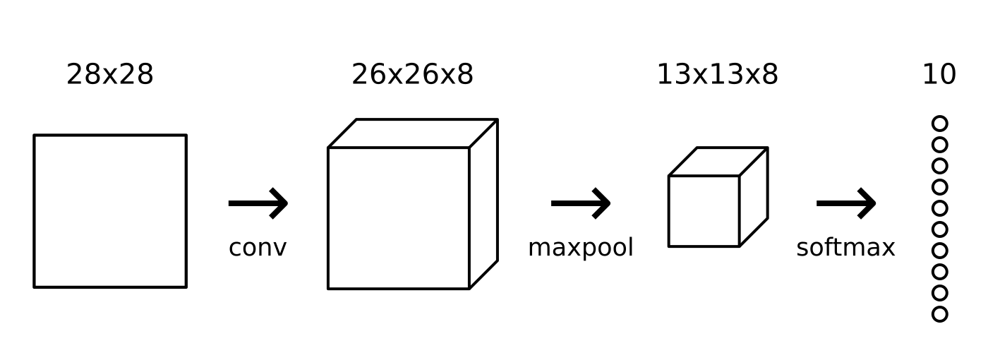
])The Sequential constructor takes an array of Keras Layers. We’ll use 3 types of layers for our CNN: Convolutional, Max Pooling, and Softmax.

This is the same CNN setup we used in my introduction to CNNs. Read that post if you’re not comfortable with any of these 3 types of layers.
from tensorflow.keras.layers import Conv2D, MaxPooling2D, Dense, Flatten

num_filters = 8
filter_size = 3
pool_size = 2

model = Sequential([
  Conv2D(num_filters, filter_size, input_shape=(28, 28, 1)),
  MaxPooling2D(pool_size=pool_size),
  Flatten(),
  Dense(10, activation='softmax'),
])num_filters,filter_size, andpool_sizeare self-explanatory variables that set the hyperparameters for our CNN.- The first layer in any
Sequentialmodel must specify theinput_shape, so we do so onConv2D. Once this input shape is specified, Keras will automatically infer the shapes of inputs for later layers. - The output Softmax layer has 10 nodes, one for each class.
4. Compiling the Model
Before we can begin training, we need to configure the training process. We decide 3 key factors during the compilation step:
- The optimizer. We’ll stick with a pretty good default: the Adam gradient-based optimizer. Keras has many other optimizers you can look into as well.
- The loss function. Since we’re using a Softmax output layer, we’ll use the Cross-Entropy loss. Keras distinguishes between
binary_crossentropy(2 classes) andcategorical_crossentropy(>2 classes), so we’ll use the latter. See all Keras losses. - A list of metrics. Since this is a classification problem, we’ll just have Keras report on the accuracy metric.
Here’s what that compilation looks like:
model.compile(
  'adam',
  loss='categorical_crossentropy',
  metrics=['accuracy'],
)
Onwards!
5. Training the Model
Training a model in Keras literally consists only of calling fit() and specifying some parameters. There are a lot of possible parameters, but we’ll only supply these:
- The training data (images and labels), commonly known as X and Y, respectively.
- The number of epochs (iterations over the entire dataset) to train for.
- The validation data (or test data), which is used during training to periodically measure the network’s performance against data it hasn’t seen before.
There’s one thing we have to be careful about: Keras expects the training targets to be 10-dimensional vectors, since there are 10 nodes in our Softmax output layer. Right now, our train_labels and test_labels arrays contain single integers representing the class for each image:
import mnist

train_labels = mnist.train_labels()
print(train_labels[0]) # 5
Conveniently, Keras has a utility method that fixes this exact issue: to_categorical. It turns our array of class integers into an array of one-hot vectors instead. For example, 2 would become [0, 0, 1, 0, 0, 0, 0, 0, 0, 0] (it’s zero-indexed).
Here’s what that looks like:
from tensorflow.keras.utils import to_categorical

model.fit(
  train_images,
  to_categorical(train_labels),
  epochs=3,
  validation_data=(test_images, to_categorical(test_labels)),
)
We can now put everything together to train our network:
import numpy as np
import mnist
from tensorflow.keras.models import Sequential
from tensorflow.keras.layers import Conv2D, MaxPooling2D, Dense, Flatten
from tensorflow.keras.utils import to_categorical

train_images = mnist.train_images()
train_labels = mnist.train_labels()
test_images = mnist.test_images()
test_labels = mnist.test_labels()

# Normalize the images.
train_images = (train_images / 255) - 0.5
test_images = (test_images / 255) - 0.5

# Reshape the images.
train_images = np.expand_dims(train_images, axis=3)
test_images = np.expand_dims(test_images, axis=3)

num_filters = 8
filter_size = 3
pool_size = 2

# Build the model.
model = Sequential([
  Conv2D(num_filters, filter_size, input_shape=(28, 28, 1)),
  MaxPooling2D(pool_size=pool_size),
  Flatten(),
  Dense(10, activation='softmax'),
])

# Compile the model.
model.compile(
  'adam',
  loss='categorical_crossentropy',
  metrics=['accuracy'],
)

# Train the model.
model.fit(
  train_images,
  to_categorical(train_labels),
  epochs=3,
  validation_data=(test_images, to_categorical(test_labels)),
)
Running that code on the full MNIST dataset gives us results like this:
Epoch 1
loss: 0.2433 - acc: 0.9276 - val_loss: 0.1176 - val_acc: 0.9634
Epoch 2
loss: 0.1184 - acc: 0.9648 - val_loss: 0.0936 - val_acc: 0.9721
Epoch 3
loss: 0.0930 - acc: 0.9721 - val_loss: 0.0778 - val_acc: 0.9744
We achieve 97.4% test accuracy with this simple CNN!
6. Using the Model
Now that we have a working, trained model, let’s put it to use. The first thing we’ll do is save it to disk so we can load it back up anytime:
model.save_weights('cnn.h5')We can now reload the trained model whenever we want by rebuilding it and loading in the saved weights:
from tensorflow.keras.models import Sequential
from tensorflow.keras.layers import Conv2D, MaxPooling2D, Dense, Flatten

num_filters = 8
filter_size = 3
pool_size = 2

# Build the model.
model = Sequential([
  Conv2D(num_filters, filter_size, input_shape=(28, 28, 1)),
  MaxPooling2D(pool_size=pool_size),
  Flatten(),
  Dense(10, activation='softmax'),
])

# Load the model's saved weights.
model.load_weights('cnn.h5')
Using the trained model to make predictions is easy: we pass an array of inputs to predict() and it returns an array of outputs. Keep in mind that the output of our network is 10 probabilities (because of softmax), so we’ll use np.argmax() to turn those into actual digits.
# Predict on the first 5 test images.
predictions = model.predict(test_images[:5])

# Print our model's predictions.
print(np.argmax(predictions, axis=1)) # [7, 2, 1, 0, 4]

# Check our predictions against the ground truths.
print(test_labels[:5]) # [7, 2, 1, 0, 4]
8. Extensions
There’s much more we can do to experiment with and improve our network - in this official Keras MNIST CNN example, they achieve 99 test accuracy after 15 epochs. Some examples of modifications you could make to our CNN include:
Network Depth
What happens if we add or remove Convolutional layers? How does that affect training and/or the model’s final performance?
model = Sequential([
  Conv2D(num_filters, filter_size, input_shape=(28, 28, 1)),
  Conv2D(num_filters, filter_size),  MaxPooling2D(pool_size=pool_size),
  Flatten(),
  Dense(10, activation='softmax'),
])
Dropout
What if we tried adding Dropout layers, which are commonly used to prevent overfitting?
from tensorflow.keras.layers import Dropout
model = Sequential([
  Conv2D(num_filters, filter_size, input_shape=(28, 28, 1)),
  MaxPooling2D(pool_size=pool_size),
  Dropout(0.5),  Flatten(),
  Dense(10, activation='softmax'),
])
Fully-connected Layers
What if we add fully-connected layers between the Convolutional outputs and the final Softmax layer? This is something commonly done in CNNs used for Computer Vision.
from tensorflow.keras.layers import Dense
model = Sequential([
  Conv2D(num_filters, filter_size, input_shape=(28, 28, 1)),
  MaxPooling2D(pool_size=pool_size),
  Flatten(),
  Dense(64, activation='relu'),  Dense(10, activation='softmax'),
])
Convolution Parameters
What if we play with the Conv2D parameters? For example:
# These can be changed, too!
num_filters = 8
filter_size = 3

model = Sequential([
  # See https://keras.io/layers/convolutional/#conv2d for more info.
  Conv2D(
    num_filters,
    filter_size,
    input_shape=(28, 28, 1),
    strides=2,    padding='same',    activation='relu',  ),
  MaxPooling2D(pool_size=pool_size),
  Flatten(),
  Dense(10, activation='softmax'),
])
Conclusion
You’ve implemented your first CNN with Keras! We achieved a test accuracy of 97.4% with our simple initial network. I’ll include the full source code again below for your reference.
Further reading you might be interested in include:
- My Keras for Beginners series, which has more Keras guides.
- The official getting started with Keras guide.
- My post on deriving backpropagation for training CNNs.
- More posts on Neural Networks.
Thanks for reading! The full source code is below.
The Full Code
# The full CNN code!
####################
import numpy as np
import mnist
from tensorflow.keras.models import Sequential
from tensorflow.keras.layers import Conv2D, MaxPooling2D, Dense, Flatten
from tensorflow.keras.utils import to_categorical

train_images = mnist.train_images()
train_labels = mnist.train_labels()
test_images = mnist.test_images()
test_labels = mnist.test_labels()

# Normalize the images.
train_images = (train_images / 255) - 0.5
test_images = (test_images / 255) - 0.5

# Reshape the images.
train_images = np.expand_dims(train_images, axis=3)
test_images = np.expand_dims(test_images, axis=3)

num_filters = 8
filter_size = 3
pool_size = 2

# Build the model.
model = Sequential([
  Conv2D(num_filters, filter_size, input_shape=(28, 28, 1)),
  MaxPooling2D(pool_size=pool_size),
  Flatten(),
  Dense(10, activation='softmax'),
])

# Compile the model.
model.compile(
  'adam',
  loss='categorical_crossentropy',
  metrics=['accuracy'],
)

# Train the model.
model.fit(
  train_images,
  to_categorical(train_labels),
  epochs=3,
  validation_data=(test_images, to_categorical(test_labels)),
)

# Save the model to disk.
model.save_weights('cnn.h5')

# Load the model from disk later using:
# model.load_weights('cnn.h5')

# Predict on the first 5 test images.
predictions = model.predict(test_images[:5])

# Print our model's predictions.
print(np.argmax(predictions, axis=1)) # [7, 2, 1, 0, 4]

# Check our predictions against the ground truths.
print(test_labels[:5]) # [7, 2, 1, 0, 4]