
The main data structure that you’ll use in NumPy is the N-dimensional array. An array can have one or more dimensions to structure your data. In some programs, you may need to change how you organize your data within a NumPy array. You can use NumPy’s reshape() to rearrange the data.
The shape of an array describes the number of dimensions in the array and the length of each dimension. In this tutorial, you’ll learn how to change the shape of a NumPy array to place all its data in a different configuration. When you complete this tutorial, you’ll be able to alter the shape of any array to suit your application’s needs.
In this tutorial, you’ll learn how to:
- Change the shape of a NumPy array without changing its number of dimensions
- Add and remove dimensions in a NumPy array
- Control how data is rearranged when reshaping an array with the
orderparameter - Use a wildcard value of
-1for one of the dimensions inreshape()
For this tutorial, you should be familiar with the basics of NumPy and N-dimensional arrays. You can read NumPy Tutorial: Your First Steps Into Data Science in Python to learn more about NumPy before diving in.
Supplemental Material: Click here to download the image repository that you’ll use with NumPy reshape().
Install NumPy
You’ll need to install NumPy to your environment to run the code in this tutorial and explore reshape(). You can install the package using pip within a virtual environment. Select either the Windows or Linux + macOS tab below to see instructions for your operating system:
It’s a convention to use the alias np when you import NumPy. To get started, you can import NumPy in the Python REPL:
>>> import numpy as np
Now that you’ve installed NumPy and imported the package in a REPL environment, you’re ready to start working with NumPy arrays.
Understand the Shape of NumPy Arrays
You’ll use NumPy’s ndarray in this tutorial. In this section, you’ll review the key features of this data structure, including an array’s overall shape and number of dimensions.
You can create an array from a list of lists:
>>> import numpy as np
>>> numbers = np.array([[1, 2, 3, 4], [5, 6, 7, 8]])
>>> numbers
array([[1, 2, 3, 4],
       [5, 6, 7, 8]])
The function np.array() returns an object of type np.ndarray. This data structure is the main data type in NumPy.
You can describe the shape of an array using the length of each dimension of the array. NumPy represents this as a tuple of integers. The array numbers has two rows and four columns. Therefore, this array has a (2, 4) shape:
>>> numbers.shape
(2, 4)
You can represent the same data using a different shape:
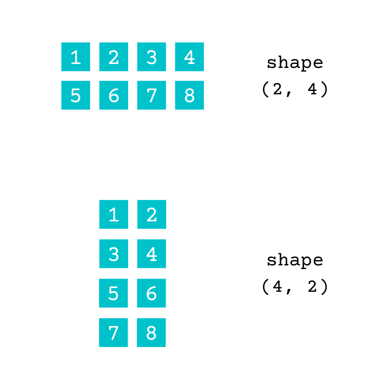
Both of these arrays contain the same data. The array with the shape (2, 4) has two rows and four columns and the array with the shape (4, 2) has four rows and two columns. You can check the number of dimensions of an array using .ndim:
>>> numbers.ndim
2
The array numbers is two-dimensional (2D). You can arrange the same data contained in numbers in arrays with a different number of dimensions:
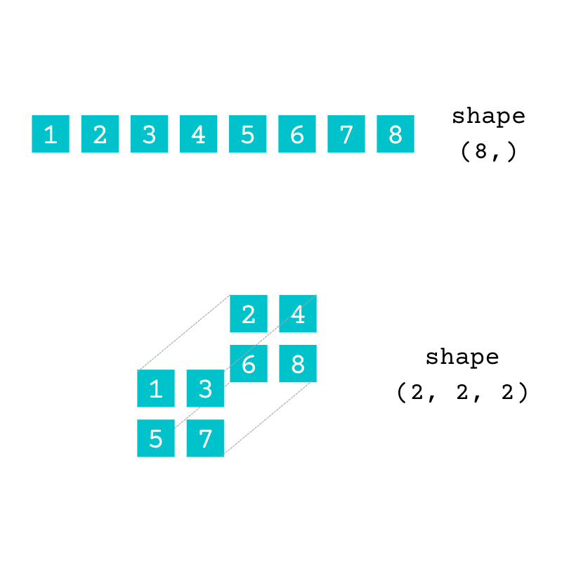
The array with the shape (8,) is one-dimensional (1D), and the array with the shape (2, 2, 2) is three-dimensional (3D). Both have the same data as the original array, numbers.
You can use the attribute .shape to understand the array’s characteristics:
- Number of dimensions: The length of the tuple
.shapeshows you how many dimensions are in the array. For example,(2, 4)contains two items, which means that an array with this shape is a 2D array. - Length of each dimension: The integers in
.shaperepresent the length of each dimension in the array. For example, if the shape of an array is(2, 4), then the first dimension has a length of 2 and the second dimension has a length of 4.
You can use the information contained in the tuple .shape to understand the structure of the arrays that you’re working with.
NumPy’s reshape() allows you to change the shape of the array without changing its data. You can reshape an array into a different configuration with either the same or a different number of dimensions.
In the following sections, you’ll work through several short examples that use reshape() to convert arrays from one shape into another.
Change an Array’s Shape Using NumPy reshape()
NumPy’s reshape() enables you to change the shape of an array into another compatible shape. Not all shapes are compatible since all the elements from the original array needs to fit into the new array.
You can use reshape() as either a function or a method. The documentation for the function shows three parameters:
ais the original array.newshapeis a tuple or an integer with the shape of the new array. Whennewshapeis an integer, the new array will have one dimension.orderenables you to determine how the data is configured in the new array.
You’ll use the first two parameters in this section. You’ll learn about order later in this tutorial.
When using reshape() as a method of np.ndarray, you no longer need to use the first parameter, a, since the object is always passed to the method as its first argument. You’ll use reshape() as a method in the rest of this tutorial. However, everything you learn about this method also applies to the function.
Note: A method is a function defined inside a class body. You call reshape() as a function using np.reshape(a, newshape). The equivalent method call is a.reshape(newshape).
In this section of the tutorial, you’ll explore NumPy’s reshape() through an example. You need to write code to help a school’s head of computing, who needs to transform some data.
There are five classes in the same grade level, with ten pupils each. A 2D array stores the anonymized test results for each student. The shape of the array is (5, 10). The five rows represent the classes, and each row has the test score for each student in the class.
You can re-create a version of this array using random values. You can generate random values in NumPy by using the default_rng() generator and then calling one of its methods. In this example, you call .integers():
>>> import numpy as np
>>> rng = np.random.default_rng()
>>> results = rng.integers(0, 100, size=(5, 10))
>>> results
array([[53, 28, 33, 23, 81, 58, 16,  6, 91, 84],
       [ 4, 20, 20, 27, 27, 82, 19, 76, 57, 47],
       [56, 97, 53, 21, 72, 18, 91, 29, 38, 15],
       [85, 20, 30, 67, 65,  1, 52, 95, 87, 70],
       [66, 70,  9, 30, 73,  1, 56, 29, 10, 76]])
The .integers() method creates uniformly distributed random integers in the range defined by the first two arguments. The third argument, size, sets the shape of the array. The uniform distribution of integers is convenient for this example, but you can also use other distributions.
The head of computing analyzed the results of each class separately and now wants to convert the array into a single row containing all the results to continue working on the year as a whole.
One option is to convert the array with five rows and ten columns into a new array with one row and fifty columns. You can achieve this using reshape():
>>> year_results = results.reshape((1, 50))
>>> year_results
array([[53, 28, 33, 23, 81, 58, 16,  6, 91, 84,  4, 20, 20, 27, 27, 82,
        19, 76, 57, 47, 56, 97, 53, 21, 72, 18, 91, 29, 38, 15, 85, 20,
        30, 67, 65,  1, 52, 95, 87, 70, 66, 70,  9, 30, 73,  1, 56, 29,
        10, 76]])

>>> year_results.shape
(1, 50)
>>> year_results.ndim
2
You pass the tuple (1, 50) as an argument, and it’s assigned to the parameter newshape. The first ten items in year_results are the test scores for the students in the first class. The second class’s results follow these, and so on.
Warning: You shouldn’t reshape an array by setting the value of the attribute .shape. Although this works for now, it’s discouraged and may be deprecated in the future. Use reshape() instead.
Although year_results only has one row, it’s still a 2D array in NumPy. You can confirm this in a number of ways:
- The attribute
year_results.shapeis a tuple with two values. - The attribute
year_results.ndimhas a value of 2. - When
year_resultsis displayed, there are two pairs of square brackets.
If you want to access the first test score in this array, then you’ll need to use both row and column indices since year_results is a 2D array:
>>> year_results[0]
array([53, 28, 33, 23, 81, 58, 16,  6, 91, 84,  4, 20, 20, 27, 27, 82, 19,
       76, 57, 47, 56, 97, 53, 21, 72, 18, 91, 29, 38, 15, 85, 20, 30, 67,
       65,  1, 52, 95, 87, 70, 66, 70,  9, 30, 73,  1, 56, 29, 10, 76])

>>> year_results[0, 0]
53
When you use a single index, as in year_results[0], the index 0 refers to the row. You access the first element using year_results[0, 0].
Reduce an Array’s Number of Dimensions
When you use reshape(), the new array doesn’t need to have the same number of dimensions as the original one. You can reshape the original results array from earlier into a 1D array:
>>> year_results = results.reshape((50,))
>>> year_results
array([53, 28, 33, 23, 81, 58, 16,  6, 91, 84,  4, 20, 20, 27, 27, 82, 19,
       76, 57, 47, 56, 97, 53, 21, 72, 18, 91, 29, 38, 15, 85, 20, 30, 67,
       65,  1, 52, 95, 87, 70, 66, 70,  9, 30, 73,  1, 56, 29, 10, 76])

>>> year_results.shape
(50,)
>>> year_results.ndim
1

>>> year_results[0]
53
The new array now has one dimension of length 50. When you want to access one of its values, you only need a single index.
The shape of a 1D array is a tuple with one item. You can also use an integer as an argument for reshape() when you want a 1D array:
>>> year_results = results.reshape(50)
>>> year_results
array([53, 28, 33, 23, 81, 58, 16,  6, 91, 84,  4, 20, 20, 27, 27, 82, 19,
       76, 57, 47, 56, 97, 53, 21, 72, 18, 91, 29, 38, 15, 85, 20, 30, 67,
       65,  1, 52, 95, 87, 70, 66, 70,  9, 30, 73,  1, 56, 29, 10, 76])

>>> year_results.shape
(50,)
When you pass an integer argument for the parameter newshape, you get the same result as when you pass a tuple with a single element. However, note that the attribute .shape is still a tuple with one element and not an integer.
You reduced the number of dimensions of the array from two to one without removing any of the data from the original array.
Increase an Array’s Number of Dimensions
In this section, you’ll work on a new example. You installed a temperature sensor that records the house’s temperature every three hours. The sensor outputs a 1D NumPy array with all the readings.
You’ll use random values to represent the temperature readings in this example:
>>> import numpy as np
>>> rng = np.random.default_rng()
>>> temperatures = rng.normal(18, 1, size=200)
>>> temperatures
array([17.78916577, 18.48720738, 17.16745854, 18.63306583, 18.30034365,
       18.36342512, 18.37339031, 19.22000687, 17.14534477, 15.90837538,
       17.37115548, 17.68445145, 19.20665509, 16.86856826, 19.15139203,
       ...
       18.17433295, 17.46510906, 18.30706081, 16.47186073, 14.49601283,
       19.36982869, 18.78297168, 17.30458478, 18.40410989, 18.41390098,
       16.77663847, 17.4153006 , 17.83923996, 18.77606957, 18.68240767])

>>> temperatures.shape
(200,)
>>> temperatures.ndim
1
You call rng.normal() to get a normal distribution with a mean temperature of 18 degrees Celsius and a standard deviation of 1 degree Celsius. The resulting array has one dimension since the size argument isn’t a tuple but a single integer. You’ll reshape this array into different configurations in the following sections of this tutorial.
You want to rearrange the data so that each 24-hour period is in a separate row of the array. Each row will have eight temperature readings since the sensor records a value every three hours.
The temperatures array contains 200 readings which means that the reshaped array should have 25 rows each containing eight values:
>>> temperatures_day = temperatures.reshape((25, 8))
>>> temperatures_day
array([[17.78916577, 18.48720738, 17.16745854, 18.63306583, 18.30034365,
        18.36342512, 18.37339031, 19.22000687],
       [17.14534477, 15.90837538, 17.37115548, 17.68445145, 19.20665509,
        16.86856826, 19.15139203, 14.9819749 ],
       [17.09155469, 18.55311155, 17.82173679, 16.44808271, 18.33660455,
        16.39911841, 17.46262617, 16.11580479],
       ...
       [19.27637947, 18.53564103, 18.7538117 , 17.28817758, 15.99178148,
        16.7630879 , 18.25401129, 18.5474829 ],
       [17.46122335, 18.17433295, 17.46510906, 18.30706081, 16.47186073,
        14.49601283, 19.36982869, 18.78297168],
       [17.30458478, 18.40410989, 18.41390098, 16.77663847, 17.4153006 ,
        17.83923996, 18.77606957, 18.68240767]])

>>> temperatures_day.shape
(25, 8)
>>> temperatures_day.ndim
2
The original array’s first eight temperature readings make up the first row in the reshaped array. The following eight temperatures are stored in the second row of temperatures_day, and so on.
You can access the readings for a single 24-hour period more easily with this 2D array. For example, you can extract the readings for the second day using temperatures_day[1]:
>>> temperatures_day[1]
array([17.14534477, 15.90837538, 17.37115548, 17.68445145, 19.20665509,
       16.86856826, 19.15139203, 14.9819749 ])
When you use the index 1, you get the 1D array, which is in the second place in temperatures_day.
You used NumPy reshape() to increase the number of dimensions of the original array from one to two, keeping all the data in the correct order. In the next section, you’ll explore what happens when the shape of the new array isn’t compatible with the original.
Ensure the Shape of the New Array Is Compatible With the Original Array
You decide you would also like to organize your data into weeks, and you want to reshape the array into three dimensions:
- The first dimension represents the weeks.
- The second dimension represents the days within a week.
- The third dimension represents the individual readings within a day.
Each week includes 56 temperature readings since there are eight readings each day and seven days a week. Therefore, the complete set of 200 readings isn’t divisible into a whole number of weeks. There are three full weeks, but that leaves extra readings from part of the fourth week.
You can attempt to reshape the array to include three weeks of data by passing the tuple (3, 7, 8) to reshape(). However, this will fail:
>>> temperatures_week = temperatures.reshape((3, 7, 8))
Traceback (most recent call last):
  ...
ValueError: cannot reshape array of size 200 into shape (3,7,8)
This raises an error since an array of shape (3, 7, 8) contains 168 elements. The original array with 200 values can’t fit into this new array.
You can reshape an array if the dimensions of the new array are compatible with those of the original one. To create an array of shape (3, 7, 8) you can trim the original data to the first 168 values:
>>> days_per_week = 7
>>> readings_per_day = 8
>>> number_of_weeks = len(temperatures) // (days_per_week * readings_per_day)
>>> number_of_weeks
3

>>> trimmed_length = number_of_weeks * days_per_week * readings_per_day
>>> trimmed_length
168

>>> temperatures_week = temperatures[:trimmed_length].reshape(
...     (number_of_weeks, days_per_week, readings_per_day)
... )

>>> temperatures_week
array([[[17.78916577, 18.48720738, 17.16745854, 18.63306583,
         18.30034365, 18.36342512, 18.37339031, 19.22000687],
        [17.14534477, 15.90837538, 17.37115548, 17.68445145,
         19.20665509, 16.86856826, 19.15139203, 14.9819749 ],
        ...
        [18.56767078, 17.86123831, 18.81186461, 18.69086946,
         18.45513019, 17.99669896, 18.20703493, 18.06268867],
        [17.11528709, 18.83735551, 16.49220439, 17.10466892,
         17.88975427, 18.44527053, 16.71681421, 18.26859973]],

       [[18.24864303, 18.63744622, 18.80297891, 15.43544626,
         18.29333932, 18.52391081, 17.09935544, 18.40424394],
        [17.64065163, 18.38806208, 18.40054375, 16.63639914,
         17.8642428 , 19.04086886, 16.76040209, 17.87085502],
        ...
        [18.64131675, 18.21219446, 16.8594998 , 17.56934664,
         17.17678561, 17.56550433, 18.51482721, 19.20758859],
        [19.24228543, 17.14736191, 18.30302811, 17.12356338,
         18.31287005, 19.14701069, 17.53495458, 18.8801354 ]],

       [[18.154868  , 16.81175022, 19.22848909, 17.8604165 ,
         17.86463829, 19.11074667, 18.24322805, 16.54989167],
        [17.91524201, 19.32497959, 17.43219577, 18.17353934,
         18.26306481, 19.27815777, 18.13648414, 18.27392718],
        ...
        [17.95081736, 17.24806278, 17.36949169, 17.43922213,
         19.14574375, 17.5418501 , 17.26565033, 17.47016249],
        [16.12557219, 18.49384214, 19.53422956, 16.80504269,
         17.31254144, 18.95745599, 19.46544502, 18.1389923 ]]])

>>> temperatures_week.shape
(3, 7, 8)
>>> temperatures_week.ndim
3
You’ve increased the number of dimensions of the original array from one to three using reshape(). In this example, you had to remove some of the original data to achieve the required shape.
If you don’t want to discard any of the data, then you can extend the original array instead of trimming it. You’ll need to choose a value to fill in the additional places in the extended array. In this example, you’ll use NumPy’s Not a Number constant, .nan. This constant is suitable since any numeric value that you use could be mistaken for a temperature value:
>>> extended_length = (number_of_weeks + 1) * (
...     days_per_week * readings_per_day
... )
>>> extended_length
224

>>> additional_length = extended_length - len(temperatures)
>>> additional_length
24

>>> temperatures_extended = np.append(
...     temperatures, np.full(additional_length, np.nan)
... )
>>> len(temperatures_extended)
224

>>> temperatures_extended
array([17.78916577, 18.48720738, 17.16745854, 18.63306583, 18.30034365,
       18.36342512, 18.37339031, 19.22000687, 17.14534477, 15.90837538,
       17.37115548, 17.68445145, 19.20665509, 16.86856826, 19.15139203,
       ...
       18.17433295, 17.46510906, 18.30706081, 16.47186073, 14.49601283,
       19.36982869, 18.78297168, 17.30458478, 18.40410989, 18.41390098,
       16.77663847, 17.4153006 , 17.83923996, 18.77606957, 18.68240767,
               nan,         nan,         nan,         nan,         nan,
               nan,         nan,         nan,         nan,         nan,
               nan,         nan,         nan,         nan,         nan,
               nan,         nan,         nan,         nan,         nan,
               nan,         nan,         nan,         nan])
You work out how many values you need to add to the array to fill a whole number of weeks. The extended array temperatures_extended is the result of using np.append() to add an array full of np.nan values to temperatures. You use np.full() to create the array with np.nan values.
Now you can reshape the extended array into the shape that you need to have four weeks of data:
>>> temperatures_week = temperatures_extended.reshape(
...     (number_of_weeks + 1, days_per_week, readings_per_day)
... )
>>> temperatures_week
array([[[17.78916577, 18.48720738, 17.16745854, 18.63306583,
         18.30034365, 18.36342512, 18.37339031, 19.22000687],
        [17.14534477, 15.90837538, 17.37115548, 17.68445145,
         19.20665509, 16.86856826, 19.15139203, 14.9819749 ],

        ...

        [        nan,         nan,         nan,         nan,
                 nan,         nan,         nan,         nan],
        [        nan,         nan,         nan,         nan,
                 nan,         nan,         nan,         nan]]])

>>> temperatures_week.shape
(4, 7, 8)
>>> temperatures_week.ndim
3
The new array, temperatures_week, now has the shape (4, 7, 8). The values in the final week in the array with no temperature data are filled with np.nan.
When you want to reshape an array into a new shape that’s not compatible with the original one, you’ll need to decide whether you prefer to trim an array or extend it with filler values.
Control How the Data Is Rearranged Using order
In the examples that you’ve worked on so far, the reshaped arrays always had the data configured correctly. For example, the first eight values in the 1D array temperatures were rearranged into the first row of the 2D array temperatures_day. This first row represents the first day of data collection.
There will be cases where the default rearranged configuration doesn’t match your requirements. You’ll see an example of this situation in this tutorial section and learn how to use the optional parameter order in NumPy’s reshape() to obtain the configuration you need.
Explore the order Parameter
NumPy’s reshape() has an optional parameter, order, which allows you to control how the data is rearranged when you reshape an array. This parameter can accept either "C", "F", or "A" as an argument. You can start by creating a simple array and then explore the first two of these arguments:
>>> import numpy as np
>>> numbers = np.array([1, 2, 3, 4, 5, 6, 7, 8])
>>> numbers
array([1, 2, 3, 4, 5, 6, 7, 8])
>>> numbers.shape
(8,)
>>> numbers.ndim
1

>>> numbers.reshape((2, 4), order="C")
array([[1, 2, 3, 4],
       [5, 6, 7, 8]])

>>> numbers.reshape((2, 4), order="F")
array([[1, 3, 5, 7],
       [2, 4, 6, 8]])
The new arrays both have two rows and four columns. However, the elements are rearranged in different configurations.
The string arguments "C" and "F" represent the programming languages C and Fortran. These languages use different versions of array indexing:
- C uses the row-major order of indexing.
- Fortran uses the column-major order of indexing.
These terms originally refer to how elements are stored in memory in an array. However, the memory configuration isn’t relevant when using either "C" or "F" as an argument for order. The order of the indices refers to the sequential order of all the elements in the array. You can think of this as the order in which you would read out all the elements.
In the row-major order, the sequence of elements goes along rows first. Once you reach the end of the row, you’ll continue from the beginning of the next row.
In the column-major order, the sequence of elements goes down the columns first. Once you reach the end of a column, you’ll continue from the top of the next column.
You can visualize this difference with the following diagram:
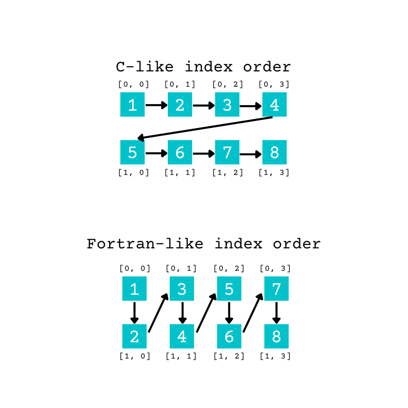
This diagram shows the different order of elements in a 2D array. You can extend the same concept to higher-dimensional arrays.
In the example above, when you pass "C" as an argument for order, the elements from the original array fill the new array using the C-like, or row-major, order. The first four elements fill the first row of the new array. When the first row is full, the remaining items start filling the second row.
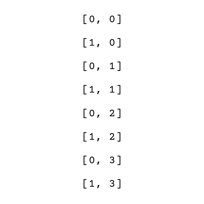
Therefore, reshape() converts the original array’s eight elements to the new array in the following order of indices when using order="C":
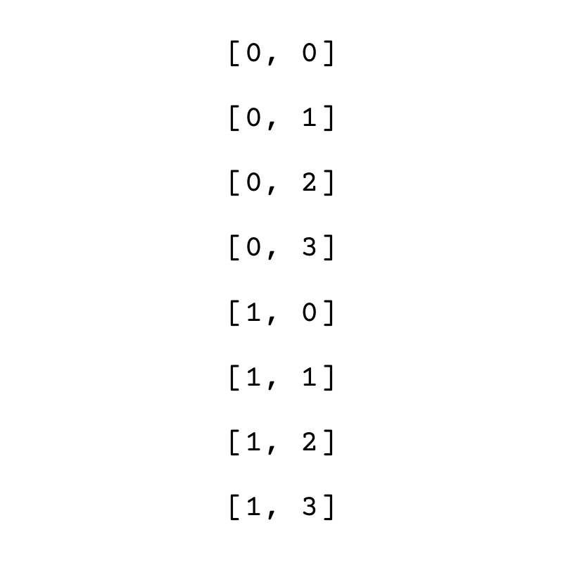
This diagram shows the order of the indices when you use C-like indexing.
With reshape(), the final axis is the quickest to change as elements are read and written. The last index changes for each successive element, but the first index only changes after four elements, when a row is complete.
When you pass "F" as an argument, reshape() uses the Fortran-like, or column-major, order. The columns are filled first.
Therefore, reshape() converts the original array’s eight elements to the new array in the following order of indices when using order="F":
This diagram shows the order of the indices when you use Fortran-like indexing.
In this case, the first index is changing faster because it changes for each successive element. The second index changes once each column is complete.
Although the different indexing orders originally represent the memory configuration of the array, the result of reshape() doesn’t depend on the actual memory configuration when you use "C" and "F" as arguments for order.
There’s a third option in addition to "C" and "F". If you pass "A" to the parameter order, then the index order will match the memory layout of the array. In most cases, you’re not aware of the the memory layout of the arrays in your program because you rely on the NumPy package to take care of these details for you. This is one of the benefits of using NumPy. Therefore, "C" and "F" are the arguments you’re most likely to need.
Reduce a Three-Dimensional Color Image to Two Dimensions
In this section, you’ll read a color image into a 3D NumPy array and create a triptych showing the red, green, and blue components side by side in a 2D image.
You’ll use the Pillow library to read the image and convert it to a NumPy array. You can install the library to your virtual environment using pip:
You can use the image file poppy.jpg (image credit) provided with this tutorial or your own image if you prefer. You’ll need to place the file in the project folder that you’re working in. If you’d like to use the provided image, then download the supplemental materials by clicking below:
Supplemental Material: Click here to download the image repository that you’ll use with NumPy reshape().
Start by reading the image file using Pillow and converting it to a NumPy array. You can also display the image using Pillow:
>>> import numpy as np
>>> from PIL import Image
>>> with Image.open("poppy.jpg") as photo:
...     image_array = np.array(photo)
...

>>> photo.show()
>>> image_array.shape
(769, 1280, 3)
>>> image_array.ndim
3
The photo.show() call will display the image using your default software for viewing images:

As this is a color image, it’s converted to a 3D NumPy array when you pass photo as an argument to np.array(). The first two dimensions represent the width and height of the image in pixels. The third dimension represents the red, green, and blue channels. Some images may also include the alpha value in the third dimension.
You want to convert this 3D array into a 2D image with the same height as the original image and three times the width so that you’re displaying the image’s red, green, and blue components side by side. Now see what happens when you reshape the 3D array. You can extract the height and width of the image in pixels by unpacking image_array.shape and discarding the third dimension:
>>> height, width, _ = image_array.shape
>>> height
769
>>> width
1280

>>> triptych = image_array.reshape((height, 3 * width))
>>> triptych.shape
(769, 3840)
>>> triptych.ndim
2

>>> Image.fromarray(triptych).show()
You reshape the 3D array into two dimensions and show the image. However, this isn’t the image that you were aiming for:

The default argument for order is "C". This means that when rearranging the 3D array, reshape() changes the last axis fastest. The last axis is the one that represents the three color channels.
Therefore, when populating the new array, reshape() first takes the red channel’s value for the image’s top-left pixel. Then it takes the green channel’s value for the same pixel and places it next to the red value. The next element in the new array is the blue channel’s value for the first pixel in the original color image.
The first three pixels in the first row of the new image all come from the first pixel of the original color image. Each pixel in the image is stretched out horizontally using its red, green, and blue values.
You can see this by zooming in on a section of the image using .crop() from the Pillow library:
>>> Image.fromarray(triptych).crop((400, 300, 500, 400)).show()
You use .crop() to select a small region of the original image. This shows a section of the image containing part of a red flower and the blue sky:

The portion of the image containing the sky has a strong blue component, while the portion of the image with the flower has a strong red component. If you follow a column in this cropped image from top to bottom, then you’ll see the brightest values shift sideways as you move from a sky portion to a flower portion of the image.
This observation confirms that each pixel in the original image is represented by its red, green, and blue components side by side in this reshaped 2D version.
However, if reshape() followed a different order and the third axis was the one that changed last, then you’d get a different image. This is the Fortran-like index order, which you can achieve by passing "F" to the order parameter:
>>> triptych = image_array.reshape((height, 3 * width), order="F")
>>> Image.fromarray(triptych).show()
You use the argument "F" when you call reshape(). The image now has the three color channels side by side:

The image on the left shows the red channel from the original image. The brightest pixels are the ones that represent the flowers’ petals. These petals are red in the original image. You can contrast this with the image on the right, which is the blue channel. The brightest pixels correspond to portions of the image showing the sky, and the pixels representing the petals are dark in the blue channel.
In this example, you’ve seen how the order in which you reshape an array can significantly impact the result. You can use the order parameter in NumPy’s reshape() to control how the data is rearranged when reshaping the array.
Use -1 as an Argument in NumPy reshape()
In all the examples that you’ve used in this tutorial, you always included the lengths of all the dimensions in the reshaped array. But if you want, you can include a wildcard option for one of the dimensions and let reshape() infer the length of the rest of the information.
You can use the same temperatures array that you used earlier, or you can re-create a new one if you’re working in a new REPL session:
>>> import numpy as np
>>> rng = np.random.default_rng()
>>> temperatures = rng.normal(18, 1, size=200)
>>> temperatures
array([17.78916577, 18.48720738, 17.16745854, 18.63306583, 18.30034365,
       18.36342512, 18.37339031, 19.22000687, 17.14534477, 15.90837538,
       17.37115548, 17.68445145, 19.20665509, 16.86856826, 19.15139203,
       ...
       18.17433295, 17.46510906, 18.30706081, 16.47186073, 14.49601283,
       19.36982869, 18.78297168, 17.30458478, 18.40410989, 18.41390098,
       16.77663847, 17.4153006 , 17.83923996, 18.77606957, 18.68240767])

>>> temperatures.shape
(200,)
There are eight readings in each 24-hour period. Earlier, you’ve manually divided 200 by 8 to determine there should be 25 rows in the reshaped array.
However, you can use the value -1 as the length for the first dimension when reshaping:
>>> temperatures_day = temperatures.reshape((-1, 8))
>>> temperatures_day
array([[17.78916577, 18.48720738, 17.16745854, 18.63306583, 18.30034365,
        18.36342512, 18.37339031, 19.22000687],
       [17.14534477, 15.90837538, 17.37115548, 17.68445145, 19.20665509,
        16.86856826, 19.15139203, 14.9819749 ],
       [17.09155469, 18.55311155, 17.82173679, 16.44808271, 18.33660455,
        16.39911841, 17.46262617, 16.11580479],
       ...
       [19.27637947, 18.53564103, 18.7538117 , 17.28817758, 15.99178148,
        16.7630879 , 18.25401129, 18.5474829 ],
       [17.46122335, 18.17433295, 17.46510906, 18.30706081, 16.47186073,
        14.49601283, 19.36982869, 18.78297168],
       [17.30458478, 18.40410989, 18.41390098, 16.77663847, 17.4153006 ,
        17.83923996, 18.77606957, 18.68240767]])

>>> temperatures_day.shape
(25, 8)
You pass a tuple with -1 as its first element. A negative number can’t be a valid length for a dimension. The value of -1 is used to let reshape() work out the length of the remaining dimension. You can use any negative number as a wildcard value, although it’s best to use -1 as described in the documentation.
You can only replace one of the dimensions with -1. You’ll get an error if you include -1 more than once:
>>> temperatures_day = temperatures.reshape((-1, -1))
Traceback (most recent call last):
  ...
ValueError: can only specify one unknown dimension
This code raises a ValueError since the argument that you pass to reshape() contains more than one occurrence of -1. There isn’t enough information to infer the length of the two unknown dimensions.
You can use this wildcard option to flatten an array with any number of dimensions. You flatten an array when you collapse it to a single dimension:
>>> rng = np.random.default_rng()
>>> numbers = rng.integers(1, 100, (2, 4, 3, 3))
>>> numbers.shape
(2, 4, 3, 3)
>>> numbers.ndim
4

>>> numbers_flattened = numbers.reshape(-1)
>>> numbers_flattened
array([76, 58, 14, 44, 15, 28, 19, 12, 18, 26, 64, 82, 20, 85, 54, 80, 26,
       18, 90, 24,  9, 61, 40, 55, 14, 81, 53, 33, 26, 40, 70, 50, 94, 46,
       30, 21, 58, 71, 79, 84, 67, 34, 93, 71, 94, 68, 59, 85, 78, 82,  9,
       36, 28, 76, 78, 27,  4, 46, 24, 99, 96, 82, 60, 67, 40, 63,  5, 69,
       15, 69, 11, 97])

>>> numbers_flattened.shape
(72,)
>>> numbers_flattened.ndim
1
You create an array named numbers, with four dimensions. The attribute numbers.ndim confirms the number of dimensions. The flattened array is a 1D array with a length of 72. The length of the new 1D array is the product of the lengths of all four dimensions in the original array.
Note: For an alternate approach, check out the Flattening Python Lists for Data Science With NumPy.
You can use the -1 value to make your code more flexible since you don’t need to know the length of one of the dimensions of the reshaped array.
Conclusion
Now you’re ready to start manipulating your N-dimensional arrays by rearranging the data into arrays with different shapes. You can increase or decrease the number of dimensions or reshape the array keeping the same number of dimensions.
In this tutorial, you’ve learned how to:
- Change the shape of a NumPy array without changing its number of dimensions
- Add and remove dimensions in a NumPy array
- Control how data is rearranged when reshaping an array with the
orderparameter - Use a wildcard value of
-1for one of the dimensions inreshape()
NumPy’s reshape() allows you to reconfigure any array. Using it effectively will make your work with NumPy quicker and more efficient. You’re ready to keep experimenting with reshaping arrays!
Supplemental Material: Click here to download the image repository that you’ll use with NumPy reshape().


