Combining R and Python with {reticulate} and Quarto

The R versus Python debate has been going on for as long as both languages have existed. I’m not one to takes sides - I think you need to use the best tool for the job. Sometimes R will be better. Sometimes Python will be better. But what happens if you need both languages in the same workflow? Do you need to choose? No, is the simple answer. You can use both. This blog post will show you how you can combine R and Python code in the same analysis using {reticulate} and output the results using Quarto.

What is Quarto?

Quarto is an open-source scientific and technical publishing system that lets you combine narrative text with code to create reproducible and elegantly formatted output. If you’re familiar with R Markdown, Quarto might sound somewhat similar - you can think of Quarto as next generation of R Markdown. The great thing about Quarto is that it doesn’t just support code written in R - it supports other languages, including Python!

Quarto documents have two main sections: (i) the YAML header, where we specify document-wide properties such as the output format, and (ii) the content, which can include text, images, code, and more. For the example in this blog post, I’m going to output the code and results from the analysis to revealjs slides so my YAML header looks like this:

1
2
3
4
5
6
7

---
title: "Modelling lemur weights with R and Python"
author: "Nicola Rennie"
format:
  nr-revealjs:
    embed-resources: true
---

Your YAML might look a little different if you don’t have a custom theme (another blog post on customising Quarto outputs will be on the way shortly!):

1
2
3
4
5
6
7

---
title: "Modelling lemur weights with R and Python"
author: "Nicola Rennie"
format: 
  revealjs:
    embed-resources: true
---

If you want to output them to a PDF instead, then change the format argument in the YAML to be pdf:

1
2
3
4
5

---
title: "Modelling lemur weights with R and Python"
author: "Nicola Rennie"
format: pdf
---

What is {reticulate}?

The {reticulate} R package provides an interface between R and Python which allows you to call Python code within R and translate between R and Python objects.

Using {reticulate} means that your Python code can access objects created in R, and vice versa. It means you can include Python code within an R package. It means you can run Python code in the RStudio IDE console.

Using R and Python together

So let’s see an example of how we can use R and Python within the same analysis workflow. We’re going to read in a data set using R, fit a linear model in Python, then plot the residuals using {ggplot2} in R (and output our analysis as a set of slides).

First of all, we need some data. For this example, we’re going to use the lemur data set. You can download the data from the #TidyTuesday repository. This data set gives information on different lemurs living at Duke Lemur Center, including their ages and weights measured over time. In this blog post, we’re going to look at the relationship between the age and weight of lemurs.

Within our Quarto document, we start off with an R code block that reads in the data:

1
2
3
4
5
6
7

```{r}
#| label: read-data
#| echo: true
#| message: false
#| cache: true
lemurs <- readr::read_csv('https://raw.githubusercontent.com/rfordatascience/tidytuesday/master/data/2021/2021-08-24/lemur_data.csv')
```

Here, we’ve set four options for the code block: (i) labelled the code block with label: read-data, (ii) set echo: true to make my code show in the output, (iii) set message: false to make sure the messages from read_csv() don’t show in the output, and (iv) set cache: true to cache the reading in of the data since the data set is reasonably large.

Now, we can include a second R code block to perform some data wrangling:

 1
 2
 3
 4
 5
 6
 7
 8
 9
10
11
12
13
14
15
16

```{r}
#| label: wrangling
#| echo: true
#| message: false
#| output-location: slide
library(dplyr)
library(knitr)
lemur_data <- lemurs %>% 
  filter(taxon == "ECOL",
         sex == "M",
         age_category == "adult") %>% 
  select(c(age_at_wt_mo, weight_g)) %>% 
  rename(Age = age_at_wt_mo, 
         Weight = weight_g)
kable(head(lemur_data))
```

Here, we’ve selected only adult male collared brown lemurs, and chosen only the columns we want to model: age and weight. Setting output-location: slide puts the table we generate onto the following slide (since the code takes up most of the space on the slide).

So far, this has all been pretty standard. It’s just some R code in a Quarto document. Now, we can add a Python code block to fit a model:

 1
 2
 3
 4
 5
 6
 7
 8
 9
10
11
12
13
14

```{python}
#| label: modelling
#| echo: true
#| message: false
lemur_data_py = r.lemur_data

import statsmodels.api as sm
y = lemur_data_py[["Weight"]]
x = lemur_data_py[["Age"]]
x = sm.add_constant(x)
mod = sm.OLS(y, x).fit()
lemur_data_py["Predicted"] = mod.predict(x)
lemur_data_py["Residuals"] = mod.resid
```

The key part here is the r. on line 4 - this tells {reticulate} to look in the R code for an object called lemur_data. You can think of this line as importing your data from R to Python. Other than that, it’s pretty standard Python code. Here, we’ve kept it very simple and fitted a linear model:

$$weight_{i} = \beta_0 + \beta_1age_{i} + e_{i}$$

Obviously, R has the capabilities to fit a linear model, and for this simple example there’s no need for us to use Python. However, this illustrates how you might approach the problem, if you find yourself needing to use a particular library or model that you can only find in Python.

After we’ve fitted any type of model, we need to check the output. For linear regression, one of the most common methods of model inspection is to plot and analyse the residuals. Residuals tell us how far away a point is from the regression line. For linear models, the main assumption is that the errors are independent and normally distributed. If our data fits that assumption, we should see that:

• the residuals are symmetric above and below 0;
• we don’t see any patterns in the residuals as the predicted values increase;
• most of the points are close to 0, and there are fewer points with higher magnitude of residual.

Whilst you can plot residuals in Python quite easily, in my opinion it’s hard to beat the quality of graphics you can achieve with {ggplot2} in R. So we include a final R code block to plot the residuals:

 1
 2
 3
 4
 5
 6
 7
 8
 9
10
11
12
13
14
15
16
17
18
19
20
21

```{r}
#| label: plotting
#| echo: true
#| output-location: slide
#| message: false
#| fig-align: center
#| fig-alt: "Scatter plot of predicted and residual values for the fitted linear model."
library(reticulate)
library(ggplot2)
lemur_residuals <- py$lemur_data_py
ggplot(data = lemur_residuals,
       mapping = aes(x = Predicted,
                     y = Residuals)) +
  geom_point(colour = "#2F4F4F") +
  geom_hline(yintercept = 0,
             colour = "red") +
  theme(panel.background = element_rect(fill = "#eaf2f2",
                                        colour = "#eaf2f2"),
        plot.background = element_rect(fill = "#eaf2f2",
                                       colour = "#eaf2f2"))
```

Here, we used py$ to import our data and specify that we want to use lemur_data_py from our Python code block. Our R code block returns the following residual plot:

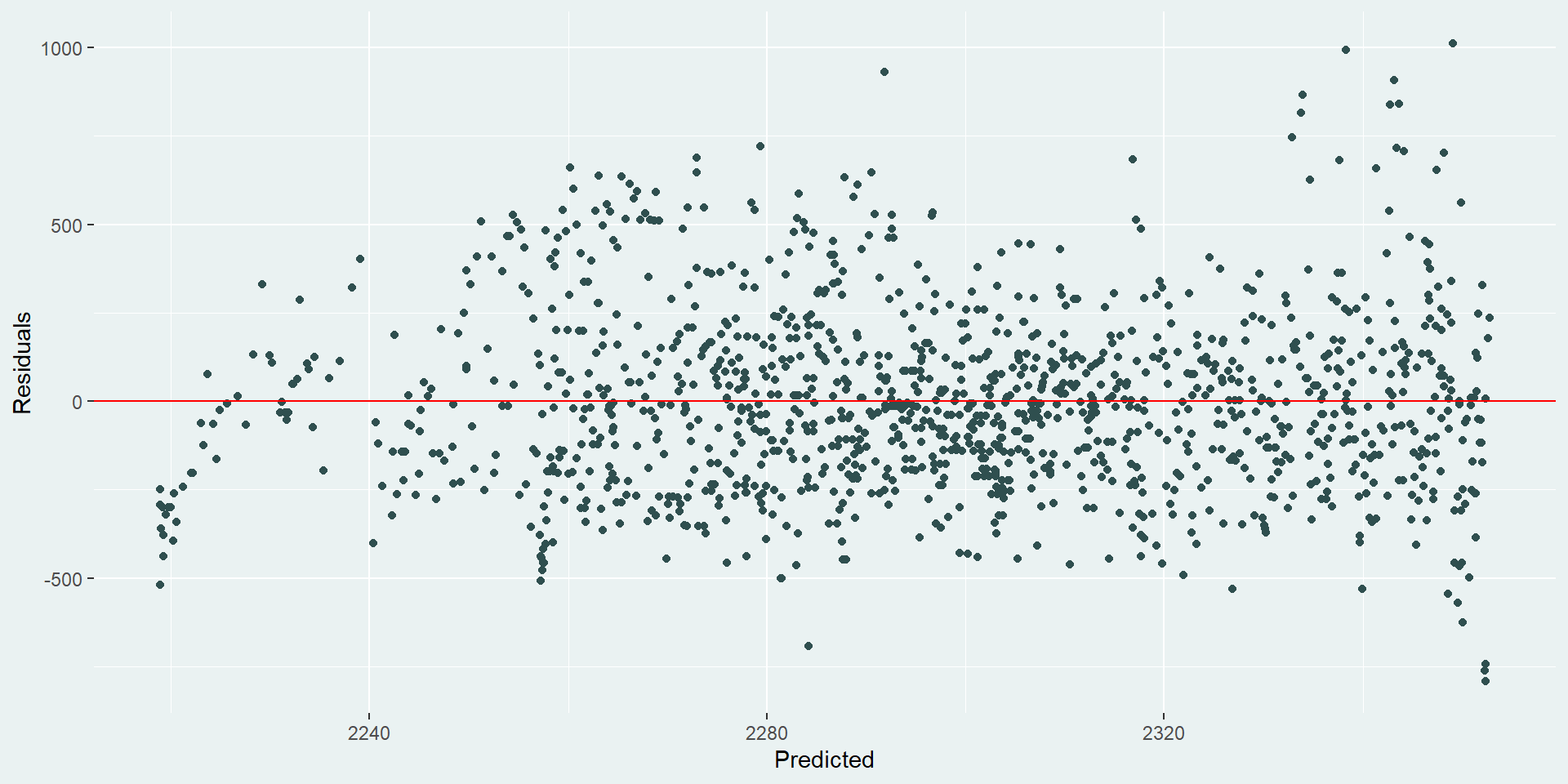
Our residuals look okay - they’re not great. It looks like there’s still some unaccounted-for trend for lemurs with smaller predicted weights. Maybe they’re not growing at a linear rate. It also looks like there is an increase in variation for lemurs with large predicted weights. It would be useful to go back and try a few other models here to see what happens, but we’ll leave that for another day…

How does it work?

There are a couple of elements to the code that means R and Python just works together. Since the document starts with an R code block, the engine used to render the document will be knitr. The rest of this blog post assumes we’re using a knitr engine, so if you’ve specified a Jupyter engine instead, this method won’t work. The Quarto documentation gives a bit more detail on how the engine is chosen. Note that these examples also work with R Markdown (not just Quarto) - although the YAML and code block options will need to be changed.

Normally, if you’re rendering a Quarto document that contains only Python code blocks, it will render using a Jupyter engine. That’s not what’s happening here. Here, the code block is still being rendered using knitr, but it knows to use {reticulate} to run the code when it finds a Python code block. In the Python code block, we accessed the data from the R code block using r.lemur_data. The r. is the key element here - it tells {reticulate} to look in the R code for an object called lemur_data and use that.

In the final R code block, we do something sort of similar to py$lemur_data_py. Here, we use py$ to specify that we want to use lemur_data_py from the Python code block. You’ll notice that we also need to explicitly call library(reticulate) for this to work (or use reticulate::py) - since it’s an R code block, {knitr} doesn’t know that it needs to use {reticulate} without us telling it to.

The final output

Let’s see what our slides containing the code, table, and plot look like…

 1
 2
 3
 4
 5
 6
 7
 8
 9
10
11
12
13
14
15
16
17
18
19
20
21
22
23
24
25
26
27
28
29
30
31
32
33
34
35
36
37
38
39
40
41
42
43
44
45
46
47
48
49
50
51
52
53
54
55
56
57
58
59
60
61
62
63
64
65
66
67
68
69
70
71
72
73
74
75
76
77
78
79
80
81
82

---
title: "Modelling lemur weights with R and Python"
author: "Nicola Rennie"
format:
  nr-revealjs:
    embed-resources: true
---

## Load the data

Load the data from the [#TidyTuesday](https://github.com/rfordatascience/tidytuesday/blob/master/data/2021/2021-08-24/readme.md) repository:

```{r}
#| label: read-data
#| echo: true
#| message: false
#| cache: true
lemurs <- readr::read_csv('https://raw.githubusercontent.com/rfordatascience/tidytuesday/master/data/2021/2021-08-24/lemur_data.csv')
```
## Data wrangling

Filter the data to only look at adult male Collared Brown Lemurs, and extract only the age and weight columns:

```{r}
#| label: wrangling
#| echo: true
#| message: false
#| output-location: slide
library(dplyr)
library(knitr)
lemur_data <- lemurs %>% 
  filter(taxon == "ECOL",
         sex == "M",
         age_category == "adult") %>% 
  select(c(age_at_wt_mo, weight_g)) %>% 
  rename(Age = age_at_wt_mo, 
         Weight = weight_g)
kable(head(lemur_data))
```

## Modelling

Fit a linear model using Python:

```{python}
#| label: modelling
#| echo: true
#| message: false
lemur_data_py = r.lemur_data

import statsmodels.api as sm
y = lemur_data_py[["Weight"]]
x = lemur_data_py[["Age"]]
x = sm.add_constant(x)
mod = sm.OLS(y, x).fit()
lemur_data_py["Predicted"] = mod.predict(x)
lemur_data_py["Residuals"] = mod.resid
```

## Plot the residuals

```{r}
#| label: plotting
#| echo: true
#| output-location: slide
#| message: false
#| fig-align: center
#| fig-alt: "Scatter plot of predicted and residual values for the fitted linear model."
library(reticulate)
library(ggplot2)
lemur_residuals <- py$lemur_data_py
ggplot(data = lemur_residuals,
       mapping = aes(x = Predicted,
                     y = Residuals)) +
  geom_point(colour = "#2F4F4F") +
  geom_hline(yintercept = 0,
             colour = "red") +
  theme(panel.background = element_rect(fill = "#eaf2f2",
                                        colour = "#eaf2f2"),
        plot.background = element_rect(fill = "#eaf2f2",
                                       colour = "#eaf2f2"))
```

You can download the .qmd file from my website.

Additional resources

You can use {reticulate} outside of Quarto (and R Markdown) documents, including to run Python code from the console in RStudio. If you want to read more about what {reticulate} can do, the package website has a lot of nice examples and guidance.

If you’re interested in using a Jupyter engine (likely if most of your code is in Python and you want to use a little bit of R), then you can do something similar using the rpy2 module.

Now you’re ready to use R and Python together!

Image: giphy.com